| Thursday, May 5 | 2:30-4:30 pm |
| Friday, May 6 | 2:30-4:00 pm |
I will have other times that I can be available by appointment. Call or email to set up a time.
| Section | Problems to do | Submit | Due date | Comments |
|---|---|---|---|---|
| 10.1 | #1-25 odd, 33,35,37,41,45,49,51,53 | 26,34 | Friday, January 21 | For Problems 49 and 51, think about completing squares. |
| Planes handout | #1-7 | 8 | Monday, January 24 | For an extra challenge, try Problems 9 and 10 on the handout. |
| 9.4 | #1-9,11,17,21,31,33 | 28 | Tuesday, January 25 | |
| 10.6 | #1-12,35,37,39,43 | 42 | Thursday, January 27 | For Problem 42 (to be submitted), include sketchs of cross-sections in addition to at least an attempt at sketching the surface as a whole. |
| 10.2 | #1-23 odd,25,29,33,39,41,43,45,49,51 | 50 | Monday, January 31 | Recall that a median in a triangle is the segment from a vertex to the midpoint of the side opposite that vertex. For Problem 49(c), you can use the fact that the medians of a triangle all intersect at a point that is two-thirds of the way along each median. |
| 10.3 | #1-7 odd,9,13,15,18,21,23,24,28 | None | None | You should now look at parts (c) and (d) of #1-7 odd. Problems #21,23, and 24 have also been added to this problem set. |
| Planes handout 2 | #1-5 | None | None | |
| 12.1 | #1,3,7,9,13-18,19,25,35,39 | 28 | Tuesday, February 8 | |
| Limit definition | #1,2 | None | None | Note that we did the first few parts of Problem 1 in class today. |
| 12.2 | #1,3,9,11,13,15,21,25,27,29,31,33,35,37,45,47 | 56 | Friday, February 11 | |
| 12.3 | #1,5,7,11,13,15,17,23,25,29,31,37,39,43,47,51,55,69,73,75 | 46 | Tuesday, February 15 | |
| 12.4 | #1,3,7,9,13,17,39,42,47,49 | 40 | Thursday, February 17 | |
| 12.5 | #1,3,5,7,9,13,15,17,19,27,29,36 | None | None | |
| 12.6 | #9,11,25,27,29,33,37,39 | 40 | Thursday, March 3 | |
| Differentials handout | #1-7 | 6 | Friday, March 4 | The problem to submit is #6 on the handout which is the same as #48 in Section 12.6. |
| 12.7 | #11,21,25,27,29,31,35,42,43,46 | 38 | Tuesday, March 8 | In the directions for Problem 42, substitute the word visualizing for imagining. |
| Applied optimization | #1-6 | 4 | Thursday, March 10 | |
| 12.8 | #3,5,11,15 | 10 | Tuesday, March 22 | |
| Nonuniform density | #1-5 | None | None | |
| 13.1 | #3,7,9,13,15,17,21,23 | None | None | |
| 13.2 | #3,9,17,25,29,33,35,47 | 40 | Thursday, March 31 | |
| Area density | #1-5 | 4 | Friday, April 1 | |
| 9.1 | #3,5,7-21 odd,23,29,41 | None | None | |
| 9.2 | #1,13,21,33,34 | None | None | |
| 13.4 | #1,3,9,11,17,19,29,31 | 30 | Monday, April 4 | |
| 13.5 | #5,11,17,25,29,35,36,39 | None | None | |
| 13.7 | #3,11,13,17,21,31,33,41,49,53,65 | None | None | |
| Volume density | #1-6 | None | None | |
| Curve integration | #1-8 | None | None | We'll address questions from these problems in class on Tuesday. |
| 10.4 | #1,3,5,15,17,27,31,33 | None | None | |
| Surface integration | #1,2,3,5 | 4 | Friday, April 22 | |
| 14.2 | #3,5,31,33,35,9,15,17,19,23,29,37 | None | None | Problems are listed in a suggested order. For Problem 23, do only the circulation and ignore flux. |
| 14.3 | #1,3,7,9,19,21,25,27,31 | 22 | Friday, April 29 | |
| Flux integrals | #1-5 | None | None | |
| Div & Curl | #1-4 | None | None | |
| Fundamental theorems | #1-4 | None | None |
Exam #5 is on Monday, May 9 from 8 to 10 am. The exam will cover material from various handouts and specific pieces of Chapter 14. See below for details. This handout has a list of specific objectives for the exam. For this exam, you can bring one sheet of notes (standard notebook size, both sides).
Below is a list of relevant handouts and corresponding subsections in the text. As I've noted previously, the approach we've taken in class differs somewhat from that of the text. In particular, the text approachs line and surface integrals strictly from a parametrization point of view. Our approach has been more geometric. In many cases, we end up parametrizing a curve (with one variable) or a surface (with two variables) without calling it this by name. In looking at the text, you might find the figures to be useful supplements to what I have been able to include in the handouts, particularly the last handout on the fundamental theorems.
If you are looking for additional practice problems, here are some suggestions:
Over the last two days, we have seen and worked a bit with various fundamental theorems of calculus, all of which have the same basic structure: Integrating the derivative of a function over a region gives the same value as integrating the function itself over the edge of the region. (In the case of a one-dimensional region such as a curve, the edge consists of only two points so integrating over the edge reduces to adding together two values.) I've added a bit of details to the handout summarizing the fundamental theorems of calculus in attempt to make this common structure more evident.
Exam #5 is on Monday, May 9 from 8 to 10 am. I will post a list of specific objectives here on Wednesday. I will also provide a list of the specific pieces of the text on which you can focus.
Today, we started with a bit of practice in computing and interpreting divergence and curl. These are the two most used derivatives of a vector field. We then saw how all of the pieces we've been developing over the past few weeks fit together into two important results: the Divergence Theorem and Stokes' Theorem. These results are fundamental theorems of calculus, all of which have the same basic structure: Integrating the derivative of a function over a region gives the same value as integrating the function itself over the edge of the region. In the case of a one-dimensional region such as a curve, the edge consists of only two points so integrating over the edge reduces to adding together two values.
This handout summarizes the fundamental theorems of calculus and has the assigned problems. The material on this is essential the same as what we saw on the slides in class.
Exam #5 is on Monday, May 9 from 8 to 10 am.
In class, we looked at two notions of derivative for a vector field: divergence and curl. There are details on these in Sections 14.4 and 14.7. These details are mingled in with other ideas. This handout pulls together the main ideas in one place.. The handout also includes the assigned problems. This handout is newly written so there may be typos. If you spot what you think is a typo, please let me know so I can check into it and make corrections as needed. Also, the handout lacks pictures so you'll need to rely on pictures we drew in class on Friday.
As you have probably sensed over the last few days, we are taking a quick trip through some big ideas. Things will come together a bit when we see how the pieces fit into the Divergence Theorem and Stokes' Theorem. Of course, we'll get only a quick look at these as well. In doing so, I'll try to be clear on what I expect you to take away from this quick tour of vector calculus.
Project #3 is due on Monday, May 2.
Today, we looked at integrating a vector field over a surface. The basic idea is adding up over the surface infinitesimal contributions of the form
The result is called a surface integral or a flux integral. Some of the ideas we use in computing a flux integral are familiar from our previous discussions about integrating a scalar field over a surface (as described on the handout Integration over a surface). As with our earlier look at surface integrals, we will take an approach that differs from that in the text. The handout Integrating a vector field over a surface has some details and an example relevant to our approach. This handout also has the assigned problems. You are also welcome to read Sections 14.5 and 14.6 in the text.
We have skipped over the ideas in Section 14.4 for now. We'll touch on these in the last few days of the course.
Project #3 is due on Monday, May 2.
Today, we discussed potential functions for vector fields and the Fundamental Theorem of Line Integrals. This FTC generalizes the familiar FTC that you learned earlier in your calculus career. Whereas any function of one variable that is continuous on an interval has an antiderivative defined on that interval, a vector field that is continuous on a region (of the plane or space) does not necessarily have a potential function. So, the FTC for line integrals is useful for integrating a vector field over a curve if there is a potential function for a region containing the curve and if we can find that potential function.
A vector field that has a potential function for a given region is said to be conservative for that region. The component test is often the easiest way to determine whether or not a vector field is conservative without directly looking for a potential function. The text states the component test using the notation \(\vec{F}=M\,\hat\imath+N\,\hat\jmath+P\,\hat{k}\). I prefer using \(\vec{F}=P\,\hat\imath+Q\,\hat\jmath+R\,\hat{k}\). In terms of this notation, the component test is stated as: A vector field \(\vec{F}=P\,\hat\imath+Q\,\hat\jmath+R\,\hat{k}\) is conservative (i.e., has a potential function) on a "nice" region if and only if \[ \frac{\partial R}{\partial y}=\frac{\partial Q}{\partial z}, \qquad \frac{\partial P}{\partial z}=\frac{\partial R}{\partial x}, \qquad\textrm{and}\qquad \frac{\partial Q}{\partial x}=\frac{\partial P}{\partial y}. \]
Another way to characterize whether or not a vector field is conservative is to ask whether or not the value of a line integral for that vector field depends on the specific curve joining the endpoints. If the value of a line integral for a vector field is path-independent for all pairs of endpoints within a given region, then the vector field is conservative.
A final way to characterize whether or not a vector field is conservative is to look at the values of line integrals over closed loops. If the value of a line integral for a vector field is zero over every closed loop in the given region, then the vector field is conservative.
For reference, here is a handout summarizing these various ways to characterize a conservative vector field.
Those of you who are or will be taking physical chemistry might want to look at the subsection "Exact Differential Forms" since this language is sometimes used in that course. A differential \(P\,dx+Q\,dy+R\,dz\) is exact if it is the result of "d-ing" a function \(V\). In other words, a differential \(P\,dx+Q\,dy+R\,dz\) is exact if there is a function \(V\) so that \(dV=P\,dx+Q\,dy+R\,dz\). The question of whether or not a differential \(P\,dx+Q\,dy+R\,dz\) is exact is equivalent to the question of whether or not the vector field \(\vec{F}=P\,\hat\imath+Q\,\hat\jmath+R\,\hat{k}\) is conservative.
Project #3 is due on Monday, May 2.
Today, we had a quick preview of the Fundamental Theorem for Line Integrals. The structure of this theorem is very similar to that of the Second Fundamental Theorem of Calculus. The details are a bit more complicated because the action is taking place in a plane or in space rather than on an interval of a number line. We'll go into the Fundamental Theorem in more detail tomorrow.
Project #3 is due on Monday, May 2.
Today, we continued discussing the idea of integrating a vector field over a curve. As with other types of integration, we can ask
The approach we will use in class differs somewhat from the approach taken in the text. You can read some details and examples about the approach we'll take in class on this handout. For homework, you should finish the problems from this worksheet that you started in class and work on the new assigned problems from Section 14.2.
Project #3 is due on Monday, May 2.
In class, we started discussing the idea of integrating a vector field over a curve. As with other types of integration, we can ask
Today, we only had time to address "What is it?" and give a very brief idea of "What does it tell us?. Tomorrow, we'll get practice in computing and use specific results to get a better feel for what this type of integration tells us. If you want a preview, you can look at this handout on integrating a vector field along a curve.
Project #3 is due on Monday, May 2.
Today, we began looking at vector fields. For much of the course, we have been working with scalar fields (without using this name). A scalar field assigns a number (i.e., a scalar) to each point in a given domain (which can be part of a line, a plane, or space). A vector field assigns a vector to each point in a given domain (which can be part of a line, a plane, or space). For the last two of the course, we will study the calculus of vector fields. Today, we got a bit of practice visualizing some basic planar vector fields on this handout. As homework, you should finish these problems and work on the assigned problems from Section 14.2. On Thursday, we will look at the idea of integrating a vector field along a curve.
In class, we looked at integrating over a surface. As with integrating over a curve, we will follow an approach that differs somewhat from the text's. Details on the approach we'll use in class on are this handout. The handout also has the assigned problems for this material. You are also welcome to read about the text's approach in Section 14.5.
Today, we first developed a new mathematical tool, namely the cross product of two vectors. The cross product of \(\vec{u}\) and \(\vec{v}\) is a new vector denoted \(\vec{u}\times\vec{v}\) and defined geometrically in relationship to the parallelogram that has \(\vec{u}\) and \(\vec{v}\) as its edges. Specfically, \(\vec{u}\times\vec{v}\) is defined geometrically by these two properties:
From this definition, it is straightforward to work out the cross product for each pair of the unit coordinate vectors \(\hat\imath\), \(\hat\jmath\), \(\hat k\). For example, \(\hat k\times\hat\imath=\hat\jmath\). Algebraic properties of the cross product include
| anticommutative property: | \(\vec{u}\times\vec{v}=-\vec{v}\times\vec{u}\) |
| distributive property: | \(\vec{u}\times(\vec{v}+\vec{w}) =\vec{u}\times\vec{v}+\vec{u}\times\vec{w}\) |
| scalar factor property: | \(\alpha(\vec{u}\times\vec{v})=(\alpha\vec{u})\times\vec{v} =\vec{u}\times(\alpha\vec{v})\) |
Using these properties and results for crossing pairs of unit coordinate vectors, we can compute the cross product of any two vectors in terms of their cartesian components. In Section 10.4 of the text, the authors show another way of computing cross products that uses determinants. You can ignore that method if you wish (particularly if you have not seen previously seen determinants.) The determinant method is essentially equivalent to the "shortcut" method we used in the example at the end of class.
Our immediate use of cross product comes in doing integration over a surface. We'll take this on next week.
Exam #4 will be on Thursday, April 14. It will cover material from Sections 13.1-13.6, 13.7, and the curve integration handout. This handout has a list of specific objectives for the exam.
If you plan to look at old exams, you might focus on the following pieces:
Here's office hours and other times I am currently available for appointments today and tomorrow:
Call or email if you'd like to arrange a time to meet outside of office hour.
As usual, I've reserved our classroom for an informal study session on Wednesday starting at 7 pm.
Today, we did another example of integrating over a curve. As noted before, The approach we will take in class to integrating over a curve differs from the approach taken in the text. This handout has some details and examples illustrating the approach we will take in class. Tomorrow, we'll address questions from the problems on this handout. You are also welcome to read Section 14.1 for the text's perspective on integration over a curve.
Exam #4 will be on Thursday, April 14. It will cover material from Sections 13.1-13.6, 13.7, and the curve integration handout. This handout has a list of specific objectives for the exam.
If you plan to look at old exams, you might focus on the following pieces:
Today, we first reviewed a geometric argument for the volume element in spherical coordinates and then we put the result to use in a few examples of setting up and evaluating an iterated integral in spherical coordinates. You'll get more practice with this in the Section 13.7 problems. The problems on the "Total from volume density" handout will give you additional practice in choosing a coordinate system in which to set and evaluate an iterated integral.
In the second half of class, we began looking at the idea of integrating over a curve. Here, we will be thinking about a curve in the plane or in space that we (conceptually) break into small pieces each of which has a length ds. In some cases, we will add up these small contributions to get the total length of the curve. In other cases, we will have a length density λ defined at each point on the curve and we will add up small contributions of the form λds to get a total (of some quantity such as charge or mass).
The approach we will take in class to integrating over a curve differs from the approach taken in the text. This handout has some details and examples illustrating the approach we will take in class. The assigned problems are on the handout. We will do more examples on Monday so you can leave these until after Monday's class if you want. You are also welcome to read Section 14.1 for the text's perspective on integration over a curve.
Exam #4 will be on Thursday, April 14.
In class, we continued discussing spherical coordinates. At the end of class, you worked through this handout to make a geometric argument for the volume element in spherical coordinates. Tomorrow, we'll put this to use in setting up iterated integrals in spherical coordinates.
I've assigned additional problems from Section 13.7. You can wait until after class tomorrow to look at these.
Exam #4 will be on Thursday, April 14.
Today, we looked at how to make a geometric argument for the volume element in cylindrical coordinates. We then introduced the idea of spherical coordinates. On Thursday, we will make a geometric argument for the volume element in spherical coordinates. We'll then be in position to set up and evaluate iterated integrals in spherical coordinates.
I have not yet assigned additional problems from Section 13.7. I'll do so after Thursday's class. In the meantime, you can look at the few problems already assigned from Section 13.7. Oh, and you can work on your project.
Project #2 is due on Thursday, April 7.
In class, we looked at an example of setting up and evaluating an iterated integral in cylindrical coordinates. You can think of cylindrical coordinates as polar coordinates r and θ for a plane together with a third coordinate z measuring the distance away from that plane. I've assigned some problems from Section 13.7. I'll assign additional problems from this section after we discuss spherical coordinates.
We will not cover the material in Section 13.6 in any detail. One of the ideas in that section is getting total mass given mass density. We have already woven that theme into our study of integration. The other ideas in Section 13.6 are center of mass and moments of inertia (aka rotational inertia). Those of you who have or are taking a first-year physics course might want to have a look at these sections to see connections between our course and your physics course.
Project #2 is due on Thursday, April 7.
Today, we looked at an example of a triple integral and the corresponding iterated integral in three variables. A triple integral involves adding up infinitely many infinitesimal contributions to a total over a region of space. To describe this type of region, we need a three-dimensional coordinate system so we end up with an iterated integral in three variables (that is, the three coordinate variables). For the example we looked at today, we used cartestian coordinates. In some other example, we might find it convenient to use some other coordinate system. Next week, we will look at two other coordinate systems for three dimensions: cylindrical coordinates and spherical coordinates.
Project #2 will be due on Thursday, April 7.
After addressing questions on area density problems and Section 9.1 problems, we looked at a few more examples of plotting polar curves. The animation below shows the curve r=cos(2θ) being traced out as θ increases. Tomorrow, we'll address questions from Section 9.2 and 13.4 problems. If this does not provide you with enough comfort using polar coordinates, we can arrange a time talk outside of class.
Many graphing calculators have a polar graphing feature. On a TI-8X, you can get to this by going to the MODE menu and choosing the option Pol from the list Func Par Pol Seq. If you then go to the Y= menu, you will see r1= where you can enter a formula for a polar curve.
Project #2 will be due on Thursday, April 7.
Today, we looked evaluating a double integral using an iterated integral in polar coordinates. To set up an interated integral in polar coordinates (r,θ), we need to do three things:
Different people will bring different levels of familiarity with polar coordinates to this course. I've assigned some problems from Sections 9.1 and 9.2 that you should start with. If you are then comfortable with polar coordinates, you can go on to the problems from Section 13.4 that deal with iterated integrals in polar coordinates.
Project #2 will be due on Thursday, April 7.
In class, we looked at a definition of double integral for a given integrand and given region of integration as a limit of a Riemann sum. If we introduce cartiesian coordinates, we can express the sum in a ways that lead to iterated integrals. Fubini's Theorem tells us that if the integrand is continuous throughout the region of integration, then the double integral and the two iterated integrals all have the same value.
Project #2 will be due on Thursday, April 7.
Today, we began looking at multivariable integration. In particular, we looked at double integrals. A double integral involves adding up infinitely many infinitesimal contributions over a two-dimensional region. A double integral of the function f over the region R is denoted \[ \iint\limits_{R}f\,dA. \] To evaluate a double integral, we will choose a coordinate system and set up an equivalent iterated integral. In cartesian coordinates, we will have either \[ \int_a^b\int_c^d f(x,y)\,dydx \qquad\textrm{or}\qquad \int_c^d\int_a^b f(x,y)\,dxdy. \] Fubini's Theorem states that if f is continuous throughout R, then \[ \iint\limits_{R}f\,dA=\int_a^b\int_c^d f(x,y)\,dydx = \int_c^d\int_a^b f(x,y)\,dxdy. \] So, we can evaluate a double integral of a continuous function by setting up and evaluating either of the corresponding iterated integrals. Each of the iterated integrals represents a particular way or organizing the "adding up" represented by the double integral. (We'll talk a bit more about the details of this on Monday.) Typically, we will evaluate an iterated integral by successively applying the Fundamental Theorem of Calculus.
If the region R is rectangular, we will have constant lower and upper bounds on both x and y. If the region is not rectangular, we will have constant lower and upper bounds on either x or y and at least one nonconstant bounds on the other one. The variable with constant bounds must be the outer variable in the iterated integral. In some cases, it is best to split the original region into smaller pieces and to then describe each piece with appropriate bounds on x and y. I've assigned problems from Sections 13.1 and 13.2 for you to get practice with both rectangular and non-rectangular regions. We'll address questions from the 13.1 problems on Monday and from the 13.2 problems on Tuesday.
In Sections 13.1 and 13.2, the authors approach double and iterated integrals within the context of computing volume for a solid region bounded by the graph of a function of two variables. This generalizes the idea of computing area for a planar region bounded by the graph of a function of one variable. In class, we will put more focus on the "total from density" interpretation/application because this context is relevant in other settings. The "area under a curve" or "volume under a surface" interpretation/application is not readily generalized to higher dimensions.
Project #2 will be due on Thursday, April 7.
Project #2 will be due on Thursday, April 7.
Exam #3 will be on Thursday March 24 from 9:30 to 10:50. It will cover material from Sections 12.6, 12.7, 12.8, and handouts since the last exam. This handout has a list of specific objectives for the exam.
I have reserved our classroom (TH 399) starting at 7 pm on Wednesday March 23 for an informal Math 280 study session. If you are looking for others to study with, come to the classroom after 7 pm and find a small group working on something of interest.
For reference, here is a handout with three approaches to solving Problem 12.8 #10.
Project #2 will be due on Thursday, April 7.
Today, we spent most of the class session addressing questions from homework problems. At the end of class, we set up an example that will involve integrating a function of two variables. We'll continue with this example tomorrow if we have time tomorrow after talking about Thursday's exam. Otherwise, we'll pick this up again on Friday.
Exam #3 will be on Thursday March 24 from 9:30 to 10:50. It will cover material from Sections 12.6, 12.7, 12.8, and handouts since the last exam.This handout has a list of specific objectives for the exam.
Project #2 will be due on Thursday, April 7.
In class, we began our discussion of integration. At a fundamental level, integration is adding up infinitely many infinitesimal contributions to a total. In your first look at integration, you probably focused on one main application, namely computing area under a curve. You can think about this as computing the area for a "rectangle with variable height". You might also have use integration to compute a total accumulation from a variable accumulation rate. In this course, we will use a third context as our primary application: using integration to compute a total amount of stuff from a density for that stuff.
Your first introduction to density (a long time ago) likely came as something like "density is mass divided by volume". Turning this around, we can say "mass is density times volume". Getting a total mass from a density by multiplication works for situations with uniform density. For nonuniform density, we will get a total from a density using integration.
In addition to generalizing to nonuniform density, 0ur use of density will be more general than your initial view in two other ways:
To denote a length density, we will typically use λ (the Greek letter "lambda"). For area density, we will generally use σ (the Greek letter "sigma"). For the more familiar volume density, we will use either ρ (the Greek letter "rho") or δ (the Greek letter "delta").
If the stuff (mass, number, charge,...) is spread out uniformly, then we can get the total amount of stuff by multiplication. If the stuff is not spread out uniformly, we need integration to compute the total amount of stuff. In class, we looked at doing this with stuff spread out on a line segment. This handout has related examples and problems.Exam #3 will be on Thursday March 24 (in the week following Spring Break).
Project #2 will be due on Thursday, April 7.
Have a great break!
Today we looked at approaching constrained optimization problems using the method of Lagrange multipliers. This method is motivated geometrically by looking for points at which a level curve/surface of the objective function is tangent to the constraint curve/surface. This is equivalent to points at which the objective function gradient vector is aligned with the constraint function gradient vector.
Exam #3 will be on Thursday March 24 (in the week following Spring Break).
Most of our time was devoted to two homework problems. At the end of class, we began looked at constrained optimization. Many applied optimization problems involve an objective function that we seek to minimize or maximize subject to a constraint equation. One way to approach a constrained optimization problem is to use the constraint equation to eliminate one of the variables in the objective function. On Thursday, we'll look at a different approach called the method of Lagrange multipliers.
Exam #3 will be on Thursday March 24 (in the week following Spring Break).
Today, you worked in groups on the first problem or two from this handout. The remaining problems are your homework assignment for today. In applied optimization problems, you must often first build the relevant function. Part of this involves identifying the relevant independent variables. In some contexts, there is a constraint that relates variables. If so, you can use the constraint to eliminate one of the variables and thus reduce the number of independent variables. Once you have built the function in terms of the truly independent variables, you can look for the relevant extreme value.
Today, we first discussed the second-derivative test. To better understand why the second-derivative test works, we put together two pieces:
We then turned our attention to global extreme values. As with local extreme values, we want to distinguish between what it is and how to find it. "What it is" for global extreme values is given by the following definition.
Definition: Given a function f:R2→R, we say an input (x0,y0) is a global maximizer and the corresponding output f(x0,y0) is a global maximum for a given region D if f(x0,y0) ≥ f(x,y) for all (x,y) in that D. Global minimizer and global minimum are defined similarly with the inequality reversed.
"How to find it" for global extreme values generally consists of putting together a list of outputs to compare. To generate this list, we need to find all critical points that are in the interior of the region D and we need to analyze the boundary of D.
In class, we looked at local extreme values. In thinking about extreme values, we want to distinguish between what it is and how to find it.
"What it is" for local extreme values is given by the following definition.
Definition: Given a function f:R2→R, we say an input (x0,y0) is a local maximizer and the corresponding output f(x0,y0) is a local maximum if there is an open disk centered at (x0,y0) such that f(x0,y0) ≥ f(x,y) for all (x,y) in that disk. Local minimizer and local minimum are defined similarly with the inequality reversed.
"How to find it" for local extreme values generally consists of two steps:
At the end of class, we did a quick example of using the second-derivative test. Tomorrow, we'll go through this idea a bit more deliberately. We'll also look at global extreme values.
I've assigned problems from Section 12.7. Most of these can wait until after class tomorrow but you might want to begin looking at the first few.
Project #1 is due on Friday March 4. If you would like an extension until Monday, March 7, just send an email asking. Come talk with me if you have questions on your work or your writing.
In class, we looked at how to use differentials to relate small changes among variables. Generally, we start with a nonlinear relation among various variables and we then compute a linear relation among the differentials for those variables. Differentials can be thought of as coordinates in the "zoomed-in world". Differentials are always related linearly. Ratios of differentials give rates of change. No limit is needed since the limit process has already been taken care of in "zooming in" process.
Working with differentials complements working with the linearization function L. Differentials are useful when we want to focus on change and rate of change. Linearizations are useful when we want to focus on approximating specific output values.
Project #1 is due on Friday March 4. Come talk with me if you have questions on your work or your writing.
In class, we reviewed tangent lines for functions of one variable and then considered tangent planes for functions of two variables. We then recast these ideas in terms of linearization. The linearization of a function f is a linear function L built using information about f at a specific point (x0,y0). If the function is differentiable at a point, then the linearization based at that point is the best linear approximation. There are many contexts in which one trades in the full accuracy of a function for the simplicity of the linearization. In making this trade, it is often essential to have some handle on how much error is introduced by trading in for the linearization. We looked at an error bound for the linearization of a function of one variable. There is a similar error bound for the linearization of a function of two variables. In class, we did not do an example of getting an upper bound on the error in a linearization for a function of two variables. I've written up the details of an example in this handout. You might find this useful in looking at Problem 33 from Section 12.6.
The text's approach to tangent planes and linearization for functions of two variables differs from what we did in class. The text starts with the more general idea of a tangent plane to a surface at a point where that surface is not necessarily the graph of a function z=f(x,y). In reading Section 12.6, you can focus on
For reference, here's the applet we looked at in class that allows you to look at tangent planes for the graph of a function of two variables.
Tomorrow, we will talk about differentials. This will provide us with a clean and powerful way to look at the linear relations that underlie linearization.
Project #1 is due on Friday March 4.
We meet in a computer lab today so you can get hands-on experience with Mathematica. Mathematica is a general purpose mathematics software system. You can think of it as a powerful graphing calculator. When it originated, Mathematicawas often to referred to as a \emph{computer algebra system (CAS)}. CAS programs are characterized by allowing for symbolic calculations in contrast to numeric calculations. The phrase CAS does not fully describe the capabilities of Mathematica or other similar programs. Other similar commercial packages include Matlab and Maple. Sage is an open source system that is being developed as a freely available alternative to commercial products. You can learn more about Sage at sagemath.org These systems have different origins but have converged to include roughly the same capabilities. Different points of origin mean each has different relative strengths and weaknesses. I have not carefully evaluated those strengths and weaknesses. I use Mathematica primarily because it is the system I learned first and now know best. I plan to seriously explore switching to Sage this summer.
If you are interested in Mathematica, you can find it on many computers on campus. (It is definitely on the computers in the Thompson Hall computer lab.) There is a small glitch in the installation of the software that points to an invalid address for something called the license server so you might get an error message if you are the first person to launch Mathematica on any particular machine. If so, you will get a dialog box with a warning about failing to connect to a license server. To fix things, press the Enter Password button in this dialog box. This will bring up a new dialog box with two options: "Single Machine License" or "Network License". Choose the "Network License" option and then enter the server name "errol.pugetsound.edu" in the box provided. That should do it. This will only need to be done once on each machine so you won't need to do it again if you return to the same computer.
You can also get to some of Mathematica's capabilities online through the Wolfram Alpha web site. (Wolfram is the company that produces Mathematica. Wolfram Alpha is a web-based service to provide information and do computations.) At the WolframAlpha site, you can enter Mathematica commands or just try natural language. Mathematica commands will be interpreted without ambiguity whereas natural language input generally has some ambiguity that might be interpreted in a way other than what you have in mind.
Next week, we'll pick up with new material starting with tangent planes and linearization. For this weekend, there is no new homework so you have time to work on Project #1 which is due on Friday March 4.
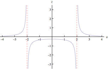
Some of you have asked about Problem 3 from the Fall 2010 Exam #2. This problem asks about continuity for the function \[ f(x,y)=\frac{1}{x^2+y^2-4}. \] Since the numerator is constant and the denominator is a polynomial, this function is continuous everywhere except where the denominator is zero. So, the only discontinuities are where \(x^2+y^2=4\). In other words, the only discontinuities are on the circle of radius 2 centered at the origin. Since the issue here is division by zero with a nonzero value in the numerator, the discontinuity is a vertical asymptote. To be specific, the graph of the function asymptotes on the cylinder \(x^2+y^2=4\). The graph asymptotes down on the inner surface of the cylinder and asymptotes up on the outer surface. Because the graph has rotational symmetry around the z-axis, we can visualize the surface by plotting the y=0 cross-section and then thinking about what surface this generates when rotated around the z-axis. The y=0 cross-section is shown below. The asymptote lines in this plot generate the asymptote cylinder when rotated around the z-axis.
Project #1 is due on Friday March 4.
Today, we had a quick look at what differentiability means for functions of two variables. We then addressed questions in preparation for Exam #2.
Exam #2 will be on Thursday February 24. We will use the 80-minute period from 9:30-10:50. The exam will cover material from Sections 12.1-12.5. This handout has a list of specific objectives for the exam.
I have reserved our classroom (TH 399) starting at 7 pm on Wednesday February 23 for a Math 280 study session. If you are looking for others to study with, come to the classroom after 7 pm and find a small group working on something of interest.
Project #1 is due on Friday March 4.
In class, we looked at the gradient operator (as part of talking about Section 12.5 #36). We also discussed the statement of Clairaut's Theorem on equality of mixed partials. This theorem gives precise conditions under which equality of mixed partial derivatives is guaranteed.
Exam #2 will be on Thursday February 24. We will use the 80-minute period from 9:30-10:50. The exam will cover material from Sections 12.1-12.5. This handout has a list of specific objectives for the exam.
Project #1 is due on Friday March 4.
Today, we looked at the idea of directional derivative. For a function f, we can ask about the rate of change at a particular point in a particular direction. We denote the directional derivative as \(df/ds\) where df represents an infinitesimal rise and ds represents an infinitesimal run. We can compute a directional derivative by finding the component of the gradient vector along the direction of interest. If the unit vector \(\hat{u}\) gives the direction of interest, then the directional derivative is given by \[ \frac{df}{ds}=\vec{\nabla} f\cdot\hat{u}. \] An alternate notation for direction derivative is \(D_{\hat{u}}f\). With this, we can write the result as \[ D_{\hat{u}}f=\vec{\nabla} f\cdot\hat{u}. \]
I have added problems to the assignment from Section 12.5 that deal with directional derivative. You can also finish the problems from the handout that you worked on in class. I've included some answers on the linked version of this handout.
Exam #2 will be on Thursday February 24. We will use the 80-minute period from 9:30-10:50.
Project #1 is due on Friday March 4.
In class, we did two things:
While the reasoning we went through to connect these two things may initially be challenging, the take-away messages are simple:
Here's a handout outlined the reasoning we discussed in class. A key part of this reasoning is that infinitesimal changes \(df\) in outputs are related to infinitesimal displacements \(d\vec{r}\) by \( df=\vec\nabla f\cdot d\vec{r}\).
The text takes a different approach to gradient vectors that starts with looking at directional derivatives. We'll talk about directional derivatives in class tomorrow. I've assigned a few probems from Section 12.5. I'll assign additional problems after class tomorrow.
Exam #2 will be on Thursday February 24. We will use the 80-minute period from 9:30-10:50.
Project #1 is due on Friday March 4.
In class, we started discussed the idea of greatest rate of change for a function of two or more variables. We start with this handout on estimating greatest rate of change for a function of two variables. Since greatest rate of change involves both direction and magnitude, we represent the greatest rate of change as a vector at each point in the domain of the function. These are called gradient vectors. So, at each point in the domain of the function, a gradient vector
To estimate a gradient vector, we can think about zooming in a point until we see level curves as a set of parallel lines. The direction of the greatest rate of change is perpendicular to these lines. We can estimate the magnitude as the ratio of an estimated "rise" and an estimated "run". As homework, you do this esimating for the points on the handout. I've added a series of "zoomed in" pictures to the linked version of the handout. Here's a view where you can control the zoom.
Tomorrow, we will see how to compute components of gradient vectors using partial derivatives. We will also see how to use a gradient vector to compute a directional derivative to get the rate of change in a specified direction.
In class, we looked at some examples of chain rules involving partial derivatives. Chain rules are relevant when differentiating functions that are compositions of other functions. In the context of functions of more than one variable, there are many ways to build compositions so there are many chain rules. Rather than trying to memorize a chain rule for each specific type of composition, you should work to understand how the pieces of a chain rule fit together in general. The text shows how to use tree diagrams as one way of doing this.
The main goal for class today was to start becoming proficient with the mechanics of computing partial derivatives. I've assigned (a lot) of problems from Section 12.3 so that you can master these mechanics. You'll need to recall all of your differentiation techniques from first-semester calculus and you'll need to keep the right mindset. For more practice, you can finish the problems from the in-class worksheet.
For reference, here is a handout on the Greek alphabet. Greek letters are frequently used in mathematics. For example, the Greek letters ε ("epsilon") and δ ("delta") are commonly used in a precise definition of limit.
In class, we looked at estimating rate of change for a function of two variables. As example, we used the relationship between T, p, and V given by the ideal gas law. On the worksheet, you used a plot of level curves for T in the Vp-plane to estimate
for a variety of points.
To get exact values for these rates of change rather than estimates, we turn to differentiation. Specifically, a partial derivative gives us the rate of change in the output variable with respect to one of the input variables with all other input variables held constant. We'll discuss this in more detail tomorrow. In the meantime, you should finish the worksheet that we began in class today.
The initial writing exercise for writing projects is due on Friday, February 11. Details about some conventional style and other issues are on the handout "Some notes on writing in mathematics".
Today, we looked at how to generalize the ideas of limit and continuity from functions of one variable to functions of two or more variable. As a starting point, we reminded ourselves of some basic definitions for functions of one variable which we then generalized to functions of two variables. One part of your homework is two problems from a handout that ask you to write out some of the details in generalizing a precise definition of limit to functions of two and three variables. The other part of your homework is problems from Section 12.2 to get practice in analyzing limits and continuity for functions of two and three variables.
The initial writing exercise for writing projects is due on Friday, February 11. Details about some conventional style and other issues are on the handout "Some notes on writing in mathematics".
In class, we spent most of our time discussing problems from Section 12.1 to gain comfort with functions of two and three variables. We ended with a brief look ahead to one notion of derivative for functions of more than one variable.
The initial writing exercise for writing projects is due on Friday, February 11. Details about some conventional style and other issues are on the handout "Some notes on writing in mathematics".
At the beginning of class, we discussed the projects that you will be doing in the course. To get started, you will do the initial writing exercise on this overview of the projects. Details about some conventional style and other issues are on the handout "Some notes on writing in mathematics". This initial writing exercise is due on Friday, February 11.
Our next focus in the course will be functions of several variables. We started today by looking at examples of functions of two variables. The usual ideas of function are relevant: domain, range, and graph. Building or visualizing a graph requires thinking in three dimensions since we need two coordinates for the inputs (x,y) and one coordinate for the output z=f(x,y). One approach to is to sketch level curves (a.ka. contours) in the input plane. A level curveis a curve in the input plane along which the output has a constant value.
For functions of three variables, we can think about domain and range. The graph of a function of three variables requires thinking in four dimensions, which we will not do directly. We can, however, draw or visualize level surfaces. A level surfaceis a surface in the input space along which the output has a constant value.
Note that we will be skipping over one last idea from Chapter 10 (namely, cross products) and all of Chapter 11 for now. We'll come back to some of this material later in the semester.
Our next focus in the course will be functions of several variables. We started today by looking at examples of functions of two variables. The usual ideas of function are relevant: domain, range, and graph. Building or visualizing a graph requires thinking in three dimensions since we need two coordinates for the inputs (x,y) and one coordinate for the output z=f(x,y). One approach to is to sketch level curves (a.ka. contours) in the input plane. A level curve in the input plane is a curve along which the output has a constant value.
Note that we will be skipping over one last idea from Chapter 10 (namely, cross products) and all of Chapter 11 for now. We'll come back to this material later in the semester.
Exam #1 will be on Thursday February 3. We will use the 80 minute period from 9:30 to 10:50. The exam will cover material from Sections 9.4, 10.1, 10,2, 10.3, 10.6 and the two handouts on equations of planes. This handout has a list of specific objectives for the exam.
I will be available for office hour today (Tuesday) from 12:30 to 1:30 and for appointments after that until at least 4:00. On Wednesday, I will be busy most of the day until 4:00. If you have questions, email or call to set up a time to talk. I can also try to address questions sent by email, although using mathematical notation is not always easy.
I have reserved our classroom (TH 399) starting at 7 pm on Wednesday February 2 for a Math 280 study session. If you are looking for others to study with, come to the classroom after 7 pm and find a small group working on something of interest.
In class, we talked about two ideas that involve the dot product. One is the idea of computing the component and projection of one vector in the direction of another vector. These two things are closely related. The component of one vector in the direction of another is a number that tells us how much one vector points along the direction of the other vector. The projection of one vector in the direction of another is a vector that gives us the piece of one vector along the direction of the other vector. The dot product is useful in computing both of these.
The other idea we discussed in class is what we will call the point-normal form for the equation of a line. The starting point for this equation is to consider specifying a plane by giving a point on the plane and a vector perpendicular to the plane. Such a vector is called a normal vector. There are details on this in Section 10.5 but these are mixed in with several other ideas so I have pulled out the main idea we want on this handout.
Exam #1 will be on Thursday February 3. We will use the 80 minute period from 9:30 to 10:50. The exam will cover material from Sections 9.4, 10.1, 10,2, 10.3, 10.6 and the two handouts on equations of planes. This handout has a list of specific objectives for the exam.
Today, we introduced the idea of the dot product of two vectors. Our approach was to start with the question of how to find the angle between two vectors if we know the components. We were able to get a nice expression for the cosine of that angle using the law of cosines. We then defined the dot product as the numerator of that expression.
In the end, we can separate out a definition of dot product that is independent of how we got to it. The dot product is an operation that takes two vectors and results in a number. In terms of components, the dot product is given by \[\vec{u}\cdot\vec{v}=u_x v_x+u_y v_y+u_z v_z.\] In terms of geometry, the dot product is given by \[ \vec{u}\cdot\vec{v}=\|\vec{u}\|\,\|\vec{v}\|\cos\theta\] where \(\theta\) is the angle between the two vectors. In many situations, you will want to think geometrically (using the second expression) and then compute in terms of components (using the first expression).
I have assigned problems from Section 10.3 that deal with dot product. Note that you can leave parts (c) and (d) of #1-7 odd until after class on Monday. Those problems will make more sense after we discuss some additional details about dot products in class.
Exam #1 will be on Thursday February 3. If possible, we will use the 80 minute period from 9:30 to 10:50. If you have not already replied to my email asking whether or not this works for your schedule, please do so as soon as possible.
In class, we continued developing basic ideas about vectors. As you begin to master (or review) these ideas, try to develop both geometric and algebraic ways of working with vectors. In many contexts, you will find it useful to get started by geometrically and then turn to components to compute.
Exam #1 will be on Thursday February 3. If possible, we will use the 80 minute period from 9:30 to 10:50. If you have not already replied to my email asking whether or not this works for your schedule, please do so as soon as possible.
Today, we began talking about vectors using displacements as an example. We gave geometric definitions of what it means to add and scale vectors. Later, we'll introduce a coordinate system and will be able to use components to add and scale vectors. Since we've just gotten started on vectors, I've only assigned one problem from Section 10.2. I'll assign more after Thursday's class.
For another view of quadric surfaces, you can go to the Interactive Gallery of Quadric Surfaces developed by Jonathon Rogness at the University of Minnesota. The plots in this gallery allow you to manipulate the cross-sections of the quadric surfaces. (Professor Rogness is also one of the creators of a cool short film called Mobius Transformations Revealed.)
If you find that you're getting bored during class, you might look at Vi Hart's math doodling videos for some inspiration.
Our focus in class today was quadric surfaces. There is a brief catalog of these on page 655 of the text. We looked at a few examples in class; you'll need to explore the others on your own as you look at homework problems. Rather than trying to memorize the catalog on page 655, it is more important to master the ability to look at cross-sections and then see how those fit into a surface. Learning the names of these quadric surfaces is helpful so you can communicate more effectively.
You can view some interactive three-dimensional pictures (similar to ones we looked at it class) at the 3D Picture Gallery.
If you are interested in improving your sketchs of quadric surfaces, you might find this handout from Sinclair Community College to be helpful.
In class, we reviewed some basics of ellipses, parabolas, and hyperbolas. In particular, we started from a purely geometric definition for each type of curve and then introduced a coordinate system to get an analytic description. In all three cases, the analytic description is a quadratic equation in two variables. As a small challenge, you can fill in the steps that we skipped over between the geometric definition and the most common form of an analytic description for an ellipse and for a hyperbola.
We can also turn this around and ask about the graph of any quadratic equation in two variables. It is a fact that the graph of any quadratic equation in two variables is an ellipse, a parabola, or a hyperbola. That is, the graph of any equation of the form
\[ Ax^2+2Bxy+Cy^2+Dx+Ey+F=0\qquad A,B,C\textrm{ not all zero} \]
is an ellipse, a parabola, or a hyperbola. You can determine which type of curve by computing \(AC-B^2\). If this quantity is positive, the graph is an ellipse. If this quantity is zero and one of D or E is nonzero, the graph is a parabola. If this quantity is negative, the graph is a hyperbola.
Note: The mathematical expressions in the previous paragraph are typeset using a system called MathJax. This should work nicely on most combinations of operating system (Windows, Mac, Linux,...) and browser (Internet Explorer, Firefox, Chrome, Safari,...). If any of the mathematical expressions above appear to not be displaying properly for you, please send me an email with some details on what OS and browser you are using.
Next week, we will bump these ideas up to three-dimensions so we will be dealing with quadratic equations in three variables and the corresponding graphs that are surfaces in space.
In class, we looked at equations of planes. In the text, this material is covered in Section 10.5 using some ideas we have not yet developed. We will soon get to those ideas, but for now you can use this handout on equations of planes. All of the ideas here are natural generalizations of equations of lines in a plane.
After class, one of you pointed out that I made a mistake in one of the examples we did with looking planes containing the surface of the table in different configurations. When the table was tilted by putting a book under the leg at one end, I miscalculated the y-slope. We estimated (crudely) a run in the y-direction of 5 units between the two ends of the table. The corresponding rise is 1 unit rather than the 4 units that I claimed in class. The lower end of the table is 3 units above the floor while the upper end is 4 units above the floor for a rise of 1 unit. With this, our estimate of the y-slope is 1/5 rather than 4/5.
In class, we began exploring three-dimensional space using cartesian coordinates. We first looked at the graph of a function of two variables, specifically z=x3y2, and then as some simpler geometric objects (such as planes). You should start working on the assigned problems from Section 10.1. As part of this, you will need to read Section 10.1 about equations of spheres in space. This is a straightforward generalization of equations of circles in a plane.
Here is an interactive plot of the function graph we looked at in class. You can rotate and zoom to look at this from various perspectives.
To get some sense of what is expected in terms of the prerequisite courses in the calculus sequence, you might find it useful to look at this Math 180 final exam and at this Math 181 final exam from the most recent times I have taught each of these courses.
You can look at exams from last few times I taught Math 280. You can use these to get some idea of how I write exams. You can use these old exams to prepare for our exams in whatever way you want. I will not provide solutions for the old exam problems but you are welcome to discuss these problems with me.
Don't assume I am going to write our exams by just making small changes to the old exams. Also note that there may be differences in order and emphasis of topics between these exams and our course.
Fall 2010
Spring 2007