| Thursday, May 5 | 2:30-4:30 pm |
| Friday, May 6 | 2:30-4:00 pm |
| Monday, May 9 | 2:30-3:30 pm |
| Tuesday, May 10 | 2:30-3:30 pm |
I will have other times that I can be available by appointment. Call or email to set up a time.
| Section | Problems to do | Submit | Target or due date | Comments |
|---|---|---|---|---|
| 1.1 | 3,5,7,8,9,15,17,19,21 | 6 | Monday, January 24 | See comment in daily note for Thursday, January 20. |
| 1.2 | 1,3,4,9,11,13,15,17,21,23,29,33,35 | 34 | Tuesday, January 25 | |
| 1.3 | 1,3,5,9,13,14,15,17,24 | None | Thursday, January 27 | You can use any relevant technology to produce slope fields. |
| 1.4 | 7,9,15 | None | Friday, January 28 | |
| 1.5 | 1,5,7,13,15,18 | 12 | Thursday, February 3 | |
| 1.6 | 3,7,11,15,19,31,39 | None | Friday, February 4 | |
| 1.7 | 3,9,11,13,15,20,21 | 16 | Monday, February 7 | |
| 1.8 | 1,3,11,17,19,21,29,33 | None | Monday, February 7 | |
| 1.9 | 5,11,15,21,22,25 | None | Tuesday, February 8 | |
| 2.1 | 8-12,15,17, 20-23 | None | Thursday, February 17 | Problems 20-23 have been added to this assignment. |
| 2.2 | 3,5,7,9,11,13,15,17,19,21,25,27 | 8 | Friday, February 18 | |
| 2.4 | 3,5,7-9,11,14,15 | None | Monday, February 21 | |
| 2.3 | 5,7,9,11,19 | None | Thursday, February 24 | |
| 3.1 | 5,9,13,15,17,25,27 | None | Thursday, February 24 | |
| 3.2 | 3,7,9,11,17,19,21 | 20 | Tuesday, March 1 | Before doing Problem 21 here, you should do Problem 15 from Section 2.3. |
| 3.3 | 3,5,7,9,13,23,25 | 20 | Monday, March 7 | |
| 3.4 | 1,3,5,7,9,11,13,15,19,21,23 | None | Monday, March 7 | |
| 3.5 | 3,7,11,16,19,23 | None | Tuesday, March 8 | |
| 3.7 | 1,3,9,11,13 | 10 | Friday, March 25 | |
| 3.8 | 5,11,17 | None | Monday, March 28 | |
| 3.6 | 1,5,7,9,13,15,21,23,31,32 | None | Thursday, March 31 | |
| 4.1 | 5,9,13,17,31,36,37,39 | None | Monday, April 4 | |
| 4.2 | 3,5,9,11,13,15,19 | None | Monday, April 4 | |
| 4.3 | 1,5,15,17,21 | None | Tuesday, April 5 | |
| 5.1 | 1,7,11,15,17,18,19,23,27,28 | 22 | Monday, April 18 | |
| 5.2 | 1,4,5,9,13,15 | None | Tuesday, April 19 | Note that #5,9,13 here match the systems in Section 5.1 #7,11,15. |
| 5.3 | 1,3,9,11,13,15 | None | Friday, April 22 | |
| 5.4 | 1,2,3,8 | None | Thursday, April 28 |
In looking at the Lorenz equations, we had a brief glimpse of chaotic behaviour. Chaos is not possible in autonomous 2×2 systems of differential equations. A nonautonomous 2×2 system can have chaotic behaviour as described in Section 5.6 of our text. Chaos is also possible in one-dimensional discrete dynamical systems. In a discrete dynamical system, the independent variable takes on only discrete values (such as the set of natural numbers). We have been studying continuous dynamical systems in which the domain of our independent variable t is all real numbers.
There are many good starting points for studying chaotic behavior. For continuous dynamical systems, one option is
In some ways, this text is a sequel to our course text. Note that Devaney is a co-author for both. Devaney has also authored a nice book on discrete dynamical systems (and fractals):
If you want something by an author other than Devaney, you might try
Finally, for a nontechnical introduction to the history and ideas of chaos, you can read
We ended class with a field trip to the Foucault pendulum. If you would like to read more about the geometry of a Foucault pendulum, you might try
Exam #4 is a take-home exam due at 2 pm on Wednesday May 11.
In looking at phase portraits for autonomous 2×2 systems, we can try to classify all possible "ultimate fates". Among the possible fates we've seen so far are
Today, we looked at some examples that indicate another possibility:
Solution curves for a 3×3 system sit in space where there is a lot more room. In the plane, a closed solution curve (or a closed union of equilibrium points joined by homonclinic/heteroclinic curves) has an "inside" and an "outside". A solution curve starting on the inside cannot enter the outside and vice versa. In space, a closed curve does not provide this type of barrier. So, there is a much richer variety of possibilities for phase portraits of n×n systems when n > 2. Today, we did a very quick overview of one historically important example, the Lorenz equations. This 3×3 system was first analyzed in depth by Edward Lorenz in his now-classic paper "Deterministic Nonperiodic Flow". In this paper, Lorenz shows the existence of solution curves that we now describe as having chaotic behavior.
Exam #4 will be a take-home exam due at 2 pm on Wednesday May 11.
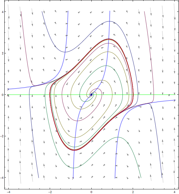
In class, you applied some of the toosl we've developed to explore a specific example. By finding the equilibrium point, analyzing the linearization there, and using nullclines to get information on the tangent vector field, you got some sense of the possible behaviors for solution curves. We got some additional insight by looking at how the radial distance changes along solution curves. Putting these clues together, we conjectured that there might be a special solution curve in the form of a periodic cycle and that solution curves starting inside that special cycle spiral out to become asymptotic from the inside while solution curves that start outside that special cycle spiral in asymptotically. We got additional supporting evidence for this conjecture by using computing technology to generate approximate solution curves. The plot below shows some of the evidence we gathered including the nullclines, tangent vectors, and some solution curves. An approximation of the limit cycle is plotted in red.
The special cycle that we conjectured exists for the system we explored is an example of a limit cycle. So, asymptotically approaching a limit cycle either from the outside or from the inside is one possible "ultimate fate" for a solution curve as t increases without bound. Other possible "ultimate fates" include asymptoting to an equilibrium point and going off to infinity. Can you think of other possible "ultimate fates" for solution curves of a 2×2 system?
Project #4 is due on Monday, May 2.
We spent most of our time today looking at Section 5.4 problems. At the end of class, we began analyzing an example that will lead us to a new idea. We'll carry on with this tomorrow.
Project #4 is due on Monday, May 2.
Last week, we saw an example of a Lyapunov function when we found that the Hamiltonian for the undamped spring model has the property of being nonincreasing along solutions of the damped spring model. Today, we looked at another example. In this case, we found a Lyapunov function by starting with a quadratic expression in the two dependent variables having some undetermined constants. By computing the rate of change in this function along solution curves, we arrived at conditions on those constants to give the desired sign of that rate of change. We then used the level curves of the Lyanpunov function to argue that the equilibrium point at the origin is a sink.
I have assigned problems from Section 5.4 that you should look at before class on Thursday. Note that we will not cover some of the ideas in Section 5.4, specifically those in the subsections "The Tuned-Mass Damper", "Gradient Systems", "General Form of Gradient Systems", and "Properties of Gradient Systems".
Project #4 is due on Monday, May 2.
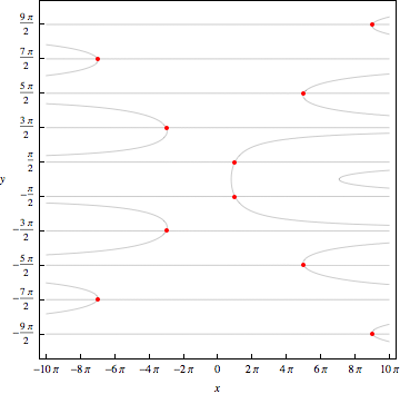
In class, we looked at the details of Section 5.3 #3, which are a bit involved. After finding the equilibrium points, we turned to computing technology for help in producing a level curve plot for the Hamiltonian. The most informative level curve plot includes the level curves that contain the equilibrium points. Below is a version for the Hamiltonian in this problem. To turn this into a phase portrait, you need to indicate directions on solution curves. To make this a bit easier, here is a version of the level curve plot that you can print out and draw directions on. You can get information about direction from the differential equations themselves.
For you reference, here are links to the Mathematica notebook I used to generate this plot:
Project #4 is due on Monday, May 2.
In class, we found a necessary condition for the existence of a Hamiltonian and did some examples. In our last example, we found a Hamiltonian for the undamped spring model. When we computed the rate of change for this Hamiltonian with respect to time along solution curves for the damped spring model, we found something of interest: The Hamiltonian is nonincreasing along solution curves for the dampled spring model. We can use this fact to get some information about those solution curves. We'll carry on with this line of reasoning next week.
I've assigned problems from Section 5.3. Try to look at all of these before class on Monday.
Project #4 is due on Monday, May 2.
Today, we analyzed a "magic" function H for our undamped pendulum model. The magical property of H is that its value is constant along solution curves for our system of differential equations. Turning this around, we can say that solution curves for our system of differential equations must lie on level curves for the function H. We spent some time deteriming the level curve structure for H. Using this together with some information from the system of equations itself, we were able to deduce that the equilibrium points (nπ,0) are centers for even values of n, a conclusion we cannot reach using the Linearization Theorem. After this, we backed up to ask how we might construct a magic function. This process should be familiar from multivariate calculus where you learned how to construct a potential function for a conservative vector field. We'll make this connection a bit more explicitly in class tomorrow.
I've assigned problems from Section 5.3. Try to look at at least some of these before class tomorrow.
Project #4 is due on Monday, May 2.
In class, we reviewed our model for the motion of a pendulum with damping and then began looking at the undamped case. For the undamped case, the Linearization Theorem does not apply at half of the equilibrium points so we need a new tool. We got a brief glimpse of this at the end of class and will see more details on Thursday.
I've assigned problems from Section 5.3. You can wait until after class on Thursday to look at these. In the meantime, you could spend time thinking about Project #4.
Project #4 is due on Monday, May 2.
Today, we set up a differential equation model for the motion of a pendulum and did some initial analysis. We'll continue this tomorrow with some focus on the undamped case.
Bring questions on Section 5.2 problems to class tomorrow.
Project #4 is due on Monday, May 2.
In class, we talked about using nullclines to split the phase plane into regions so that within each region, all tangent vectors have the same general direction. Using this with information from linearization at equilibrium points often provides enough information to determine the asymptotic nature of each solution curve.
Bring questions on Section 5.2 problems to class on Monday.
Project #4 is due on Monday, May 2.
Today, we used Section 5.1 #17 and another example to motivate the Linearization Theorem (a.k.a the Hartman-Grobman Theorem). The theorem tells us that solution curves for a nonlinear system near an equilibrium point have the same topological structure as solution curves near the origin of the linearized system provided that all eigenvalues of the linearized system have nonzero real part. Having the same topological structure means we can pick up the solution curves for the linearized system near the origin and move them, in a way that can change distances and angles but cannot involve cutting or connected curves, to be the solution curves for the nonlinear system near the equilibrium point.
Bring questions on Section 5.1 problems to class on Friday.
In class, we looked at how to linearize a nonlinear system at an equilibrium point. The linearized system gives a "zoomed in" view of what's happening near an equilibrium point. Using this view, we can classify most equilibrium point as sink, spiral sink, source, spiral source, or saddle. If the nonlinear system depends on one or more parameters, we can explore how the number, location, and nature of equilibrium points depend on the parameter values.
Bring questions on Section 5.1 problems to class on Thursday.
Today, we gathered the conjectures you made in the computer lab on Friday about features of two nonlinear systems. As part of doing this, we determing the equilibrium points analytically. We also developed a bit of language we'll use to describe features of phase portraits for nonlinear systems. Here's some quick (and somewhat informal) definitions for solution curves that "start" or "end" at equilibrium points:
We also saw some examples of separatrices (singular: separatrix). Roughly speaking, a separatrix is a solution curve that is the boundary between two categories of solution curves. Typically, the α-point and/or ω-point of solution curves on one side of the separatrix differ from the α-point and/or ω-point of solution curves on the other side.
In looking at the two examples, we also made conjectures about the nature of the phase portrait in a view that zooms in on an equilibrium point. Tomorrow, we'll start developing an analytic approach to this zooming in. This will involve linearization. At the end of class, we briefly reviewed the idea of linearization for functions of one variable. Tomorrow, we will generalize this to linearization for vector fields.
I have posted problems for Section 5.1. You can leave these until after class tomorrow.
Our goal today was to explore some nonlinear systems using computing technology. In particular, your task was to look at a nonlinear system and generate conjectures on aspects of the phase portrait such as:
On Monday, we'll begin exploring some of the features you observed in more detail using analytic tools in addition to graphical/numerical tools.
Exam #3 will be on Thursday, April 7. It will cover material from Sections 3.6-3.8 and 4.1-4.3. This handout has a list of specific objectives for the exam.
Today, we spent time interpreting our solution from Friday for an undamped spring with sinusiodal forcing. The motion of the object can be described in terms of beats that are most apparent when the driving frequency is near the natural frequency for the spring-mass system.
Exam #3 will be on Thursday, April 7. It will cover material from Sections 3.6-3.8 and 4.1-4.3. Later today or early tomorrow, I will post a list of specific objectives
In class, we looked at the last few problems from the handout on "judicious guessing" for particular solutions. Problem 7 introduces the strategy of "complexifying" a nonhomogeneous term so that we can work with exponential functions in place of sine and cosine functions. We then applied our skills and understanding to the damped spring model with external forcing. We look at generalities for the damped case and then explicitly solved in the case of a sinusiodal external forcing with no damping. On Monday, we'll spend some time interpreting the solution we came up with.
Exam #3 will be on Thursday, April 7.
Today, you got practice in "judicious guesses" for certain types of nonhomogeneous terms in a linear second-order differential equation. We'll start class tomorrow by stepping back to see what we have learned from this. We'll then apply these ideas to damped spring models with forcing.
Project #3 is due on Friday, April 1.
At the beginning of class, we looked at a connection between the system approach and the direct approach to a linear second-order differential equation. As part of this, we saw how the Wronskian can be used to analyze linear independence of a set of solutions. More details are on this optional handout on some basic theory for linear homogeneous differential equations.
We next turned attention to an example of a non-constant coefficient linear homogeneous second-order ODE. The one we looked at is an exampled of a Cauchy-Euler equation. This type of equation has power solutions rather than exponential solutions.
Finally, we began discusssing nonhomogeneous linear second-order differential equations. We'll carry on with this discussion on Thursday.
Project #3 is due on Friday, April 1.
Today, we looked at a direct approach to linear homogeneous second-order differential equations. To build the general solution to a given equation, we need two linearly independent solutions. For a constant-coefficient, we are motivated by our experience with linear systems to look for exponential solutions. Tomorrow, we'll look at an example of a non-constant coeffficent equation.
Project #3 is due on Friday, April 1.
By looking at a few examples, we got a small taste of linear 3×3 systems. The algebraic story for linear 3×3 is an obvious generalization of the 2×2 story. The geometric story is also similar but includes more variety allowed by the additional dimension.
Project #3 is due on Friday, April 1.
After going over a problem from Sectionn 3.7, we spent a bit more time discussing phase portraits for the damped spring model using the textbook software and doing some additional analysis. In particular, we looked in more detail at the eigenlines for the overdamped case.
Note that the ideas we discussed so far this week are covered in Section 3.7 of the text. Tomorrow, we'll talk about linear 3×3 systems. Next week, we'll circle back to the ideas in Section 3.6.
Project #3 is due on Friday, April 1.
Today, we used the trace-determinant view to analyze how phase portraits for a 2×2 liner system depend on a parameter. If the basic nature of the phase portraits changes at a particular parameter value, we refer to this as a bifurcation. In particular, we analyzed the basic phase portraits for the damped spring model and found four types of behavior: undamped, underdamped, critically damped, and overdamped. The critically damped case represents a transition between the underdamped case and the overdamped case. If we think of the mass m and spring constant k as fixed while the damping coefficient b varies, we have a bifurcation at the critical value of b=2√mk.
For fun, below is an animation showing the morphing phase portrait for the first example we did in class today. Note that the parameter value is displayed at the bottom of the animation. The animation loops a few times before stopping.
Note that the ideas we discussed today are covered in Section 3.7 of the text. On Thursday, we'll circle back to the ideas in Section 3.6.
Project #3 is due on Friday, April 1.
At the beginning of class, we had a brief taste of how to use linear algebra to classify a quadratic equation in two variables as an ellipse, parabola, or hyperbola. You can read more details on this optional handout. The handout includes an example of using these ideas to determine the precise geometry of the ellipse that determines the phase portrait of a 2×2 linear system with complex eigenvalues. Understanding these ideas is optional. Come talk with me outside of class if you read and have questions on the handout.
Our main goal for the day was to develop a way to understand the basic nature of the phase portrait for a 2×2 linear system without having the find the eigenvalues. We can do this by computing the trace and determinant of the coefficient matrix for the system. We'll put these ideas to use tomorrow in looking at bifurcations for a 2×2 linear system that depends on one or more parameters. For now, I've assigned one problem from Section 3.7. I'll assign additional problems after class tomorrow.
Note that the ideas we discussed yesterday and today are covered in Section 3.7 of the text. We'll soon come back to the ideas in Section 3.6.
Project #3 is due on Friday, April 1.
Today we went to the computer lab so you can get some hands-on experience with Mathematica. Using this type of computing technology is an option for the course but not required. For a freely available, open-source option, you can check out the Sage mathematics software system.
Exam #2 will be on Thursday, March 10 from 11:00 to 12:20 pm. It will cover material from Sections 2.1-2.4 and 3.1-3.5. This handout has a list of specific objectives for the exam.
Today, we looked at systems in which the coefficient matrix has a repeated eigenvalue. If there are two linearly independent eigenvectors for the repeated eigenvalue, then we get two linearly independent solutions that we can use to build the general solution for the system. If the repeated eigenvalue has only one independent eigenvector, we need to generate a second solution in some other way. Based on an example, we were motivated to look for a second solution in the form \(e^{\lambda t}(\vec{w}_0+t\vec{w}_1)\). Substituting this into the differential equation gives conditions for \(\vec{w}_0\) and \(\vec{w}_1\). You'll need to read the details on this in Section 3.5.
Exam #2 will be on Thursday, March 10 from 11:00 to 12:20 pm. It will cover material from Sections 2.1-2.4 and 3.1-3.5. This handout has a list of specific objectives for the exam.
After looking at a problem from Section 3.3, we turned to finishing the example we had started at the end of class on Thursday. We extracted two real-valued solutions from a complex-valued solution. Since the two real-valued solutions were independent, we had enough to write down the general solution to the system of equations. We then looked at visualizing the solutions we found. Each consisted of an exponential factor multiplying a vector in which each component is a linear combination of sine and cosine. In general, a vector of this form will parametrize an ellipse. With the exponential factor included, the solution is an elliptical spiral. Determining the specific geometry (orientation and size of the principal axes) of the underlying ellipse is a fun exercise in linear algebra. We'll talk briefly about this next week.
Today, we looked at some examples of solving linear 2×2 systems with complex eigenvalues. Using an eigenvalue-eigenvector pair, we can build a complex-valued solution. We can then extract the real and imaginary parts of this complex-valued solution to get two real-valued solutions. Tomorrow, we will finish up the example we were doing at the end of class and we will look at how to construct phase portraits for systems with complex eigenvalues.
Our next goal is to understand 2×2 systems for which the coefficient matrix has complex eigenvalues. As a prelude, we looked at Euler's formula and recalled some basics of complex numbers. On Thursday, we'll put these ideas to use.
Today, we looked at examples of solving and constructing phase portraits for 2×2 linear, autonomous, homogeneous systems. In the examples we looked at today, the coefficient matrix had two distinct real eigenvalues. Tomorrow, we'll start exploring examples in which the coefficient matrix has complex eigenvalues. As we explore phase portraits for 2×2 linear systems, you might find the LinearPhasePortraits piece of the textbook software to be of use.
Our goal today was to establish the basic theory for linear systems. One piece of this theory is that the solution set for a 2×2 system is a two-dimensional vector space. So, to describe all solutions for a particular system, we need only find a basis, meaning a set of two linearly independent solutions. All other solutions are linear combinations of the basis solutions. The other piece of theory tells us that we can build solutions in the form \(e^{\lambda t}\vec{v}\) where \(\lambda\) and \(\vec{v}\) are an eigenvalue-eigenvector pair for the coefficient matrix \(A\). We've seen a few examples of this. You'll see more in the problems from Section 3.2.
On Tuesday, we had a preview of some ideas that will be important in analyzing linear systems. Today, we reviewed some fundamental ideas from linear algebra. We first reviewed the definition of nonsingular matrix and the many equivalent ways of stating that a matrix is nonsingular. We then looked at the definition of eigenvalue-eigenvector pair and recalled how to find eigenvalue-eigenvector pairs. We'll carry on tomorrow by putting these linear algebra ideas to use in solving linear systems of differential equations.
We will skip over the ideas in Section 2.5 for now. The ideas are interesting and we will return to them later in the course. You might want to quickly read the section to get a sense of the main ideas.
In class, we began our systematic look at linear, homogeneous, autonomous systems \(d\vec{Y}/dt=A\vec{Y}\). We started with a partially decoupled example that we could solve without new ideas. Examining the solution lead us to the general idea of looking for solutions in the form \(e^{\lambda t}\vec{v}\) where \(\lambda\) and \(\vec{v}\) are constants. By substituting this form into the equation, we found that we do get a solution if and only if \(\lambda\) and \(\vec{v}\) are an eigenvalue-eigenvector pair for the matrix A. We'll continue exploring this idea over the next few days.
Chapter 3 of the text is written for an audience that has not necessarily seen linear algebra. (This is a typical approach for an introductory differential equations text since many colleges do not require linear algebra as a prerequisite for differential equations.) Since all of you have had linear algebra, we'll move quickly through some of the background ideas in class. You should read the text carefully and do a self-check on whether or not you understand the relevant ideas. Ask questions (e-mail, in class, in my office,...) when they arise.
In class, we looked at solving decoupled and partially decoupled systems. As part of doing this for a linear system, we highlighted the structure of the resulting solution as a linear combination of independent solutions.
Project #2 is due on Tuesday, February 22.
After a few comments about taking care with approximate solutions generated by Euler's method (and more sophisticated variants), we set up the Existence-Uniqueness Theorem for systems. This involved first defining continuously differentiable for a vector field. To be continuously differentiable at a point, all first-order partial derivatives of the component functions must be continuous in a neighborhood of that point.
Note that I have added a few problems to the Section 2.4 assignment. The new problems involve the Existence-Uniqueness Theorem.
Project #2 is due on Tuesday, February 22.
Today, we first looked at accounting for a friction or drag force in modeling the motion of an object on a spring. We then turned attention to Euler's method for systems of first-order equations. Euler's method is discussed in Section 2.4 of the text along with the Existence-Uniqueness Theorem for systems. We discuss the EUT for systems tomorrow. We'll then turn our attention to the ideas in Section 2.3.
Project #2 is due on Tuesday, February 22.
We started class with a few comments about tangent vector fields and solution curves. Tangent vector fields are useful for autonomous systems. For a system with dependent variables x and y that depend on the independent variable t, a solution give (x,y) as a function of t. We can plot this as a curve in txy-space. More often, we look at projections of this curve into the ty-plane, the ty-plane, or the xy-plane.
We next developed a model for the motion of an object on a spring. The two main elements in our model are Newton's Second Law for motion and the Hooke's law as a model for the force exerted by a spring. (Note that while both of these are labeled as "laws", the two are not on equal footing. Newton's Second Law is much more general than Hooke's law.)
I've added a few problems from Section 2.1 that deal with modeling the motion of an object attached to a spring. I've also assigned problems from Section 2.2.
If you are looking for some light entertainment, try A Case of Spring Fever. For a bit of background on the extra characters who give a running commentary mocking the original educational film, you can read about Mystery Science Theater 3000.
Project #2 is due on Tuesday, February 22.
Today, we started discussing systems of first-order differential equations. The model you examined in Project #1 is a system of four first-order ODEs for four unknown functions (R, L, E, and V each as a function of t). We'll start with the simpler situation of a 2×2 system. To provide some context, we began looking at a simple model for a predator-prey situation. For a 2×2 system, much of our analysis will be in the phase plane of the two dependent variables (R and F in our predator-prey model). The independent variable (often t) will parametrize curves in the phase plane. The phase plane generalizes the idea of a phase line for a single first-order equation.
I've assigned some problems from Section 2.1 that deal with some simple predator-prey models. Section 2.1 also has material that looks at a model for the motion of an object attached to a spring. We'll look at this idea in class next week.
Project #2 is due on Tuesday, February 22.
Exam #1 will be on Thursday February 10. We will use the 80 minute period from 11:00 to 12:20. The exam will cover material from Chapter 1 of the text. This handout has a list of specific objectives for the exam.
I have office hour from 12:30 to 1:20 today and will be available for appointments after that. On Wednesday, I have commitments until 4:00 and will then be available for appointments.
I have reserved our classroom (TH 374) starting at 7 pm on Wednesday February 9 for a Math 301 study session. If you are looking for others to study with, come to the classroom after 7 pm and find a small group working on something of interest.
In class, we looked at the idea of using an integrating factor to solve a linear first-order differential equation. In principle, we can use this approach to solve any linear first-order problem. In practice, the approach requires finding antiderivatives; in many cases, there is no nice formula for a needed antiderivative so we are left with a solution expressed in terms of an integral.
Exam #1 will be on Thursday February 10. We will use the 80 minute period from 11:00 to 12:20. The exam will cover material from Chapter 1 of the text.
Today, we looked at the structure of solutions for linear first-order differential equations. The structure parallels what you learned in linear algebra about the structure of solutions to linear systems of algebraic equations.
Section 1.8 gives examples of how to exploit structure to solve certain linear first-order equations. The techniques here are limited to specific types of coefficents a(t) and b(t). The text labels the basic ideas as "lucky guesses". It might be better to call these "educated guesses" or "judiciuous guesses" (to use the phrase from another textbook author). On Monday, we'll look at a more general (but somewhat more difficult) method for solving first-order linear equations.
Exam #1 will be on Thursday February 10. If possible, we will use the 80 minute period from 11:00 to 12:20. If you have not already replied to my email asking if this would work for you, please do so as soon as possible.
In class, we continued discussing the phase line for an autonomous first-order differential equation. We can determine the phase line structure by finding and classifying all equilibrium points.
We then turned to the question of how the phase line structure depends on any parameter that appears in the differential equation. The number, location, and nature of equilbrium points can change as the parameter is varied. A change in the number or natures of the equilibrium points is called a bifurcation.
Note that I have added a homework assignment for Section 1.7 and changed the assignment for Section 1.6. A problem from Section 1.7 is due on Monday. No problem is to be submitted from Section 1.6.
Exam #1 will be on Thursday February 10. If possible, we will use the 80 minute period from 11:00 to 12:20. If you have not already replied to my email asking if this would work for you, please do so as soon as possible.
We started class with a quick example on the "rule of thumb" for choosing a step size in Euler's method. Here is a copy of the results we looked at in class. The example is based on Section 1.4 Problem 7
We next looked at the Existence-Uniqueness Theorem. An essential factor in understanding the theorem is understanding what we mean by a solution to an initial-value problem. Declaring a domain is part of specifying a solution. In practice, a domain is often implied rather than stated explicitly. Even so, you should develop the habit of at least thinking about the domain if not writing it down explicitly.
In the last few minutes of class, we talked about phase lines for autonomous first-order differential equations. We introduced the idea of classifying each equilibrium points as a sink, a source, or a node. A sink is stable while a source or a node is unstable. One reason to study phase lines is to set up the idea of phase planes and phase space when we later study systems of first-order differential equations
Exam #1 will be on Thursday February 10. If possible, we will use the 80 minute period from 11:00 to 12:20. If you have not already replied to my email asking if this would work for you, please do so as soon as possible.
In class, we addressed questions from Section 1.4 and 1.5 problems. In the process, we discussed one aspect of Euler's method, namely how to choose a suitable step size. The trade-off in choosing a step size is between accuaracy and cost. A smaller step size means more accuracy at the cost of more computation. Here's a rule of thumb you can use in determing a reasonable step size: Repeatly calculate Euler's method approximations, cutting the step size in half each time until the change between successive approximations is smaller than the desired accuracy level.
Most of the numerical methods built into the computing technology you use will be more sophisticated than Euler's method and will generally give more accurate approximations for the same amount of computation. One of the most common methods is the fourth-order Runge Kutta method. We will not discuss the details of these more sophisticated methods in this course.
Tomorrow, we'll talk a bit more about the Existence-Uniqueness Theorem.
Exam #1 will be on Thursday February 10. If possible, we will use the 80 minute period from 11:00 to 12:20. If you have not already replied to my email asking if this would work for you, please do so as soon as possible.
Today, we talked about the issues of existence and uniqueness for solutions of initial value problems to first-order differential equations. At the end of class, I should have chosen to give a less technical version of the Existence-Uniqueness Theorem. Here's such a version:
If \(f\) and \(\displaystyle \frac{\partial f}{\partial y}\) are continuous for all points in the \(ty\)-plane near \((t_0,y_0)\), then there is a unique solution to the initial value problem \(\displaystyle\frac{dy}{dt}=f(t,y)\) with \(y(t_0)=y_0\).
This version captures the essence of the EUT but is lacking in at least two ways:
The Existence Theorem and the Uniqueness Theorem in the text give technical details that address these two deficiencies. The rectangle described in those theorems deals with the "points near \((t_0,y_0)\)" issue. The parameter \(\epsilon\) is used to describe an interval in \(t\) that serves as the domain for the solution. On Monday, we'll talk a bit more about these technical details.
Exam #1 will be on Thursday February 10. If possible, we will use the 80 minute period from 11:00 to 12:20. Look for an email from me asking whether or not this works for your schedule.
At the beginning of class, we talked briefly about some options for typesetting mathematics. If you use Microsoft Word, one option is the built-in Equation Editor that you can get to under Insert: Equation. Most mathematicians use a typesetting language called TeX (and most frequently a variant called LaTeX). The learning curve for TeX is relatively steep. If you are interested in installing a TeX system (freely available) on your computer, one place you can start is the TeX User's Group (TUG) site. Another option based on TeX is the LyX document processing system. LyX is based on TeX but has a graphical user interface so it feels more like a familiar word processor.
Our new topic for the day is Euler's method. Euler's method is a simple and straightforward process for numerically approximating a solution to an initial value problem for a first-order differential equation. Throughout the course, you will frequently use computing technology to generate numerical approximations of solutions. Studying the numerical methods built into computing technology packages is the subject of another course. We will only study Euler's method and only in enough detail to get some sense of the issues we need to keep in mind when using built-in numerical approximation methods.
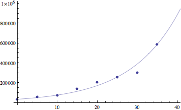
We started with a few comments on Section 1.1 #6. One issue in this problem is estimating a value for the per captia growth rate parameter k. There are many reasonable ways to do so, leading to different values of k and hence to different predictions. Reasonable approaches include
 |
 |
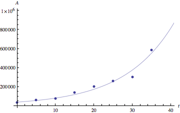 |
| With k estimated using first and second data points. | With k estimated using first and last data points. | With k estimated using regression analysis. |
We continued class by analyzing solutions for the logistic equation using both the differential equation itself and explicit solutions found using separation of variables. One of the features we found is that a solution with an initial value between 0 and the carrying capacity N will have an inflection point for y=N/2.
We then turned our attention to slope fields for first-order differential equations. You can draw a slope field by hand either by drawing tangent line segment at points on a grid or by finding isoclines (including the nullcline). There are lots of computing technology options available for producing slope fields. At the end of class, I gave you a quick look at the tool HPGSolver that is included in the software on the CD that comes with the text and at the JOde applet available online. You can use any tool with roughly equivalent functionality that you find convenient.
You should continue/start to put thought into Project #1. As you begin writing, keep in mind the style conventions and tips from Notes on writing in mathematics. On Thursday, we'll talk briefly about some options for typesetting mathematical expresssions.
If you find that you're getting bored during class, you might look at Vi Hart's math doodling videos for some inspiration.
In class, we first looked at questions on Section 1.2 problems. Then, you began working out the details of an analytic solution for the logistic equation: \[ \frac{dy}{dt}=\alpha y(1-y/N) \qquad\textrm{with}\qquad y(0)=y_0. \] As homework (not to be submitted), you should finish off the details of this. To be specific, you should
Note: The mathematical expressions on the display line above are typeset using a system called MathJax. This should work nicely on most combinations of operating system (Windows, Mac, Linux,...) and browser (Internet Explorer, Firefox, Chrome, Safari,...). If any of the mathematical expressions above appear to not be displaying properly for you, please send me an email with some details on what OS and browser you are using.
You should continue/start to put thought into Project #1. As you begin writing, keep in mind the style conventions and tips from Notes on writing in mathematics. Tomorrow, we'll talk briefly about some options for typesetting mathematical expresssions.
In class, we looked at separation of variables, a technique that works for some first-order differential equations. In using this technique, you will generally need to antidifferentiate so you'll need to recall rules, methods, and tools for this. You should be able to handle straightforward antidifferentiation "by hand". For more complicated problems, you can use a table of integrals or computing technology. This can include using online resources such as the Online Integrator or WolframAlpha.
You should put some thought into Project #1. We'll talk about writing project reports next week in class.
Today, we talked about modeling with differential equations. In particular, we developed three simple population models. The first two models were simple enough to solve explicitly. For the third model (often called the logistic model), we deduced some qualitative features of solutions without explicitly solving the differential equation.
The wording of Problems 15 in Section 1.1 is a bit muddled. Writing "harvested each year" seems to imply that the harvest happens all at once. This would be hard to model using a continuous time variable; a discrete time variable model would be more appropriate. Since we are using differential equations (and thus a continuous time variable), you should think of the harvesting as an ongoing process for these problems. You can interpret 15(a) as saying that fish are continually harvested at a rate of 100 fish per year. You can interpret 15(b) as saying that fish are continually harvested at a rate proportional to the fish population with a proportionality constant of 1/3. This is not the same as saying that we will pick a particular date and then harvest 1/3 of the fish on that date each year.
In class, we discussed a very broad overview of differential equations and then began talking about modeling with differential equations. On Thursday, we'll talk a bit more about this kind of modeling and look at a few simple examples. Before then, you should read through Section 1.1 and have a first look at some of the assigned problems.
Project #1 will be due on Monday, January 31. The project involves understanding part of the article "Reduction of HIV Concentration during Acute Infection: Independence from a Specific Immune Response", Andrew N. Phillips, Science, New Series, Vol. 271, No. 5248 (Jan. 26, 1996), pp. 497-499. (Note: This link is to the JSTOR database to which our library subscribes. If you are on the campus network, you should be able to access the article online.) The handout "Notes on writing in mathematics" has some details and tips for writing in this course.
You can look at exams from last few times I taught Math 301. You can use these to get some idea of how I write exams. You can use these old exams to prepare for our exams in whatever way you want. I will not provide solutions for the old exam problems but you are welcome to discuss these problems with me.
Don't assume I am going to write our exams by just making small changes to the old exams. Also note that there may be differences in order and emphasis of topics between these exams and our course.