Math 280B

Multivariate Calculus

Fall 2010

Homework assignments

Daily notes

Final exam week

Here are office hours for exam week:

Monday December 13	3:00-4:00 pm
Tuesday December 14	2:30-4:00 pm
Wednesday December 15	2:30-4:00 pm
Thursday December 16	2:30-4:00 pm

I will have other times that I can be available by appointment. Call or email to set up a time.

Tuesday, December 7

Our last topic for the semester is the Fundamental Theoreom of Calculus for Line Integrals (of vector fields). This FTC is only relevant for a vector field that has a potential function. This handout lists equivalent conditions for a vector field to have a potential function along with some language used in describing these conditions.

Exam #5 will be on Friday December 17 from 8:00 to 10:00 am. Note that this is the scheduled final exam period for this class.

The material for Exam #5 comes from various sections supplemented by various handouts. This handout lists the relevant topics along with the relevant text sections and handouts for each. This handout has a list of specific objectives for the exam.

You may also want to look at problems from Exam #5 Spring 2007. Problems 1-4 are relevant to the material we have covered. When looking at old exams, always keep in mind that there may be differences in emphases on topics from previous times I have taught the course. There may also be differences in notation and terminology, particularly if the text in use differs from our current text.

I have reserved TH 381 starting at 7 pm on Thursday December 16 for a Math 280 study session. If you are looking for others to study with, come to TH 381 after 7 pm and find a small group working on something of interest.

Here are office hours for the remainder of the week:

Wednesday December 8	2:30-3:30 pm
Thursday December 9	2:30-4:00 pm
Friday December 10	10:30-11:30 am and 2:30-3:30 pm

I will have other times that I can be available by appointment. Call or email to set up a time.

I will also have office hours during final exam week. I'll post a list of those office hours later this week.

Monday, December 6

Today, we discussed potential functions for vector fields and the Fundamental Theorem of Line Integrals. This FTC generalizes the familiar FTC that you learned earlier in your calculus career. Whereas any function of one variable that continuous on an interval has an antiderivative defined on that interval, a vector field that is continuous on an region (of the plane or space) does not necessarily have a potential function. So, the FTC for line integrals is useful for integrating a vector field over a curve if there is a potential function for a region containing the curve and if we can find that potential function.

A vector field that has a potential function for a given region is said to be conservative for that region. Another way to characterize whether or not a vector field is conservative is to ask whether or not the value of a line integral for that vector field depends on specific curve joining the endpoints. If the value of a line integral for a vector field is path-independent for all pairs of endpoints within a given region, then the vector field is conservative.

The component test given on page 872 of the text is generally the easiest way to determine whether or not a vector field is conservative without directly looking for a potential function. The text states the component test using the notation \(\vec{F}=M\,\hat\imath+N\,\hat\jmath+P\,\hat{k}\). I prefer using \(\vec{F}=P\,\hat\imath+Q\,\hat\jmath+R\,\hat{k}\). In terms of this notation, the component test is stated as: A vector field \(\vec{F}=P\,\hat\imath+Q\,\hat\jmath+R\,\hat{k}\) is conservative (i.e., has a potential function) on a "nice" region if and only if \[ \frac{\partial R}{\partial y}=\frac{\partial Q}{\partial z}, \qquad \frac{\partial P}{\partial z}=\frac{\partial R}{\partial x}, \qquad\textrm{and}\qquad \frac{\partial Q}{\partial x}=\frac{\partial P}{\partial y}. \]

Those of you who are or will be taking physical chemistry might want to look at the subsection "Exact Differential Forms" since this language is sometimes used in that course. A differential \(P\,dx+Q\,dy+R\,dz\) is exact if it is the result of "d-ing" a function \(V\). In other words, a differential \(P\,dx+Q\,dy+R\,dz\) is exact if there is a function \(V\) so that \(dV=P\,dx+Q\,dy+R\,dz\). The question of whether or not a differential \(P\,dx+Q\,dy+R\,dz\) is exact is equivalent to the question of whether or not the vector field \(\vec{F}=P\,\hat\imath+Q\,\hat\jmath+R\,\hat{k}\) is conservative.

Exam #5 will be on Friday December 17 from 8:00 to 10:00 am. Note that this is the scheduled final exam period for this class.

Friday, December 3

In class, we looked at integrating a vector field over a curve. This type of integral is generally called a line integral. The use of "line" here is misleading since the integration is more general than adding up over a line. We addressed three questions in class:

• Q: What is a line integral for a vector field?
  A: Adding up over a curve small contributions of the form (component of vector field tangent to curve) times (length of infinitesimal curve piece)
• Q: What is a line integral applied or interpreted?
  A: Often as work done by a force acting on an object moved along a path or as net help of fluid flow velocity in pushing a bead along a rigid wire. (This second interpretation is intuitive but not particularly precise.)
• Q: How do we compute a line integral?
  A: Build an equivalent definite integral in one variable.

Because our approach in class differs a bit from the approach taken in the textbook, I have written up some details in this handout on integrating a vector field over a curve. The handout includes some comments on notation that might help you more easily understand the problem statements for some of the assigned problems from Section 14.2. Note: The handout was updated Saturday afternoon to include a few more pictures.

In Section 14.2, you can ignore the last subsection on "Flux Across a Plane Curve".

Project #3 is due on Monday, December 6.

Exam #5 will be on Friday December 17 from 8:00 to 10:00 am. Note that this is the scheduled final exam period for this class.

Thursday, December 2

Today, we began discussing vector fields. A vector field consists of assigning (or measuring) a vector at each point in a domain (on a line, on a plane, or in space). Our focus today was on visualizing some simple vector fields in plane. We have previously seen examples of vector fields in this course without naming them as such. These examples we have seen are gradient vector fields in which the assigned vector at each point is the gradient of a given function.

In the last views days of our course, we'll have a brief look at the calculus of vector fields. (This is sometimes called vector analysis.) The calculus of vector fields is a large topic and we only have time to look at a few pieces. In particular, we will look at integrating a vector field over a curve and we'll look at one or two ways of differentiating a vector field. We'll look at the integration piece tomorrow.

In class, some of you doubted the accuracy of the Washington State map I drew. For comparison, here is the official map of the State of Washington.

Project #3 is due on Monday, December 6.

Exam #5 will be on Friday December 17 from 8:00 to 10:00 am. Note that this is the scheduled final exam period for this class.

Tuesday, November 30

Today, we looked at problems from Section 10.4 and surface integral problems. We'll have time on Thursday for another question on the surface integral problems if there is need. We'll then being discussing vector fields.

I've discovered and fixed these typos on two recent handouts:

• On Problem 5 of the curve integral problems handout, the expression \((x,y)=(t,t^2)\) should read \((x,y)=(t^2,t^3)\).
• On Problem 4 of the surface integral problems handout, the expression \(z=B\cos\phi\) should read \(z=R\cos\phi\).

Links now go to corrected versions of these handouts.

Project #3 is due on Monday, December 6.

Exam #5 will be on Friday December 17 from 8:00 to 10:00 am. Note that this is the scheduled final exam period for this class.

Monday, November 29

Today, we first developed a new mathematical tool, namely the cross product of two vectors. The cross product of \(\vec{u}\) and \(\vec{v}\) is a new vector denoted \(\vec{u}\times\vec{v}\) and defined geometrically in relationship to the parallelogram that has \(\vec{u}\) and \(\vec{v}\) as its edges. Specfically, \(\vec{u}\times\vec{v}\) is defined geometrically by these two properties:

• The direction of \(\vec{u}\times\vec{v}\) is perpendicular to the \(\vec{u}\vec{v}\)-parallelogram.
• The magnitude of \(\vec{u}\times\vec{v}\) is the area of the \(\vec{u}\vec{v}\)-parallelogram.

From this definition, it is straightforward to work out the cross product for each pair of the unit coordinate vectors \(\hat\imath\), \(\hat\jmath\), \(\hat k\). For example, \(\hat k\times\hat\imath=\hat\jmath\). Algebraic properties of the cross product include

anticommutative property:	\(\vec{u}\times\vec{v}=-\vec{v}\times\vec{u}\)
distributive property:	\(\vec{u}\times(\vec{v}+\vec{w}) =\vec{u}\times\vec{v}+\vec{u}\times\vec{w}\)
scalar factor property:	\(\alpha(\vec{u}\times\vec{v})=(\alpha\vec{u})\times\vec{v} =\vec{u}\times(\alpha\vec{v})\)

Using these properties and results for crossing pairs of unit coordinate vectors, we can compute the cross product of any two vectors in terms of their cartesian components. In Section 10.4 of the text, the authors show another way of computing cross products that uses determinants. You can ignore that method if you wish (or is you have not seen previously seen determinants.)

Our immediate use of cross product comes in doing integration over a surface. The approach we take in class differs in style from the approach taken in the text so I have written a handout with some details and examples on integration over a surface. You are also welcome, but not required, to read Section 14.5 in the text.

I have assigned problems from Section 10.5 on cross products and from this handout on integration over a surface. You should work to get mastery in computing cross products before turning to the surface integral problems. Tomorrow, we'll discuss the Section 10.5 problems and, if time permits, the curve integral problems.

Project #3 is due on Monday, December 6.

Exam #5 will be on Friday December 17 from 8:00 to 10:00 am. Note that this is the scheduled final exam period for this class.

You might find this New York Times article about an exhibit of Babylonian tablets featuring mathematics to be of interest.

Tuesday, November 23

Classes were canceled by the university today due to the weather conditions. On Monday, we'll pick up where we left off.

I have finished a draft of a handout on integrating over a curve. This handout includes the details of some examples we worked through in class last Friday and this Monday. Section 14.1 of the text covers the same ideas from a slightly different point of view. You are welcome to read Section 14.1 but you are not required to do so.

Today, I also updated the curve integration problems handout to fix a few typos that one of you pointed out. (Thanks!) One typo was in the answer for Problem 3 and the other was in the answer for Problem 8. If you spot what looks like a mistake or typo on a handout or on the course web page, let me know so I can check things out and make corrections as needed.

Project #3 is due on Monday, December 6.

Travel safely and have a great break!

Monday, November 22

Today, we looked at more examples of integration over a curve. (I have not yet drafted a handout with some notes on our approach to this. I'll do so in the next day or two and then put a link here.) You should now be able to make progress on the problems assigned from the handout.

Toward the end of class, we started discussing integration over a surface. In order to continue this discussion, we will develop a new mathematical tool called the cross product of two vectors. The cross product of \(\vec{u}\) and \(\vec{v}\) is a new vector denoted \(\vec{u}\times\vec{v}\) and defined geometrically in relationship to the parallelogram that has \(\vec{u}\) and \(\vec{v}\) as its edges. Specfically, \(\vec{u}\times\vec{v}\) is defined geometrically by these two properties:

• The direction of \(\vec{u}\times\vec{v}\) is perpendicular to the \(\vec{u}\vec{v}\)-parallelogram.
• The magnitude of \(\vec{u}\times\vec{v}\) is the area of the \(\vec{u}\vec{v}\)-parallelogram.

We'll explore cross products in more detail tomorrow. In particular, we'll figure out how to compute a cross product of two vectors if we know the components of the vectors.

In class, I distributed Project #3. This is due on Monday, December 6.

Friday, November 19

We started class with a big picture view of integration to review where we've been and preview where we're heading. We then spent a few minutes looking at a context in which integrating in higher dimensions is natural, namely integrating a probability density function (that can depend on any number of variables) to get the total probability for some event. Finally, we turned attention to our next major topic, namely integration over a curve. Here, we will be thinking about a curve in the plane or in space that we (conceptually) break into small pieces each of which has a length ds. In some cases, we will add up these small contributions to get the total length of the curve. In other cases, we will have a length density λ defined at each point on the curve and we will add up small contributions of the form λds to get a total (of some quantity such as charge or mass).

The approach we will take in class to integrating over a curve differs from the approach taken in the text. I'll write up a few notes over the weekend to post here. In the meantime, you can work on the assigned problems from this handout.

Thursday, November 18

Since you won't need to study this evening, you should consider attending the Regester Lecture to be given by Professor David Lupher of our Classics Department. Professor Lupher's talk is entitled Pagans and Pilgrims: "Beastly Practices of Mad Bacchanalians" in Early New England. More details on the topic of the talk are available here.

Tuesday, November 16

Exam #4 will be on Thursday, November 18 from 9:30 to 10:50 am. The exam will cover material from Sections 9.1, 9.2, 13.1-13.5 and 13.7 along with handouts on total from density. Note that material from Sections 13.1 and 13.2 were also covered on the previous exam. This handout has a list of specific objectives for the exam. You may also want to look at problems from Exam #4 Spring 2007. ( When looking at old exams, always keep in mind that there may be differences in emphases on topics from previous times I have taught the course. There may also be differences in notation and terminology, particularly if the text in use differs from our current text.)

I have reserved TH 381 starting at 7 pm on Wednesday November 17 for a Math 280 study session. If you are looking for others to study with, come to TH 381 after 7 pm and find a small group working on something of interest.

Since you won't need to study calculus on Thursday evening, you should consider attending the Regester Lecture to be given by Professor David Lupher of our Classics Department. Professor Lupher's talk is entitled Pagans and Pilgrims: "Beastly Practices of Mad Bacchanalians" in Early New England. More details on the topic of the talk are available here.

Monday, November 15

In class, we focused on problems from Section 13.7. I also returned Exam #3. Notes such as "EN#3A" refer to comments on this list.

Exam #4 will be on Thursday, November 18 from 9:30 to 10:50 am. The exam will cover material from Sections 9.1, 9.2, 13.1-13.5 and 13.7 along with handouts on total from density. Note that material from Sections 13.1 and 13.2 were also covered on the previous exam. This handout has a list of specific objectives for the exam. You may also want to look at problems from Exam #4 Spring 2007. ( When looking at old exams, always keep in mind that there may be differences in emphases on topics from previous times I have taught the course. There may also be differences in notation and terminology, particularly if the text in use differs from our current text.)

Since you won't need to study calculus on Thursday evening, you should consider attending the Regester Lecture to be given by Professor David Lupher of our Classics Department. Professor Lupher's talk is entitled Pagans and Pilgrims: "Beastly Practices of Mad Bacchanalians" in Early New England. More details on the topic of the talk are available here.

Friday, November 12

Today, we continued discussing spherical coordinates. As part of this, we determined the volume element in spherical coordinates. We then applied these new ideas to set up iterated integrals in spherical coordinates.

Exam #4 will be on Thursday, November 18.

Thursday, November 11

We will not cover the material in Section 13.6 in any detail. One of the ideas in that section is getting total mass given mass density. We have already woven that theme into our study of integration. The other ideas in Section 13.6 are center of mass and moments of inertia (aka rotational inertia). Those of you who have or are taking a first-year physics course might want to have a look at these sections to see connections between our course and that physics course.

Our focus today was on setting up and evaluating iterated integrals in cylindrical coordinates or spherical coordinates. We discussed the basics of cylindrical coordinates and then used these for Problem 3 on the total from volume density handout. We also began a discussion of spherical coordinates that we will finish tomorrow.

Exam #4 will be on Thursday, November 18.

Tuesday, November 9

Yesterday, we looked briefly at this handout on using the Greek alphabet in mathematics. I'm posting it here for your reference. If you're looking for some light entertainment, try translating more of the Greek words at the bottom of this handout.

In class today, we looked at more examples of setting up an iterated integral to evaluate a triple integral. The last of these was Problem 3 from the handout about total from volume density. For this, we set up an iterated integral using cartesian coordinates (x,y,z). We'll revisit this problem on Thursday. Because the cone's cross-sections parallel to the xy-plane are circles and circles are easy to describe in polar coordinates, we'll find it easier to use polar coordinates r and &theta in place of x and y. So, we will use (r,θ,z) in place of (x,y,z). The coordinates (r,θ,z) are called cylindrical coordinates.

Note that the original version of the handout about total from volume density was missing the phrase "the square of" in Problem 2. The current version has this corrected.

Exam #4 will be on Thursday, November 18.

Monday, November 8

Today, we looked at triple integrals. The essence of a triple integral is adding up small contributions to a total over a solid region of space. We often evaluated a triple integral by building an equivalent iterated integral. In class, you worked on an example of doing this using cartesian coordinates. That example is the first problem on this handout about total from volume density.

In setting up an iterating integral in cartesian coordinates, the most difficult part is often describing the solid region with bounds on x, y, and z. You can typically start by determining how the solid region projects onto one of the coordinate planes (xy, xz, or yz). Describe that projected planar region with bounds on the two relevant coordinates. Then, deduce bounds on the remaining coordinate by thinking about traversing the solid region in that third coordinate direction for a typical point in the projected planar region. In the example from class, we started by projecting the solid onto the xy-plane, got bounds on x and y to describe that planar projection, and finally deduced bounds on z.

Project #2 is due on Tuesday, November 9.

Exam #4 will be on Thursday, November 18.

Friday, November 5

In class, we went over some details on polar coordinates and then you worked on an example of evaluating a double integral by setting up the relevant iterated integral in polar coordinates. This handout has details on that example. For the weekend, you should work on problems from Sections 9.1, 9.2, and 13.4.

Project #2 is due on Tuesday, November 9.

Exam #4 will be on Thursday, November 18.

Thursday, November 4

Today, we looked evaluating a double integral using an iterated integral in polar coordinates. To set up an interated integral in polar coordinates (r,θ), we need to do three things:

• Describe the region with appropriate bounds on r and θ (with at least one of the two having constant bounds).
• Find an expression for the integrand in terms of r and θ.
• Use dA=rdrdθ or dA=rdθdr with the choice dictated by which of the variables has constant bounds.

Different people will bring different levels of familiarity with polar coordinates to this course. I've assigned some problems from Sections 9.1 and 9.2 that you should start with. If you are then comfortable with polar coordinates, you can go on to the problems from Section 13.4 that deal with double and iterated integrals.

Project #2 is due on Tuesday, November 9.

Exam #4 will be on Thursday, November 18.

Tuesday, November 2

I have changed the due date for Project #2 to Tuesday, November 9.

Monday, November 1

The original version of the handout with area density problems had a mistake in the answer for Problem 2. Here is a corrected version.

Exam #3 will be on Tuesday, November 2. We will use the 80 minute period from 8:00 to 9:20 am. The exam will cover material from Sections 12.6-12.8 (plus the handout with differentials problems) and 13.1-13.2 (plus the handouts with density problems). This handout has a list of specific objectives for the exam. You may also want to look at problems from old exams. Relevant problems include

• #7,8,9 from Exam #3 Spring 2007
• #2,4,6(a) from Exam #4 Spring 2007

When looking at old exams, always keep in mind that there may be differences in emphases on topics from previous times I have taught the course. There may also be differences in notation and terminology, particularly if the text in use differs from our current text.

I have reserved TH 381 starting at 7 pm this evening for a Math 280 study session. If you are looking for others to study with, come to TH 381 after 7 pm and find a small group working on something of interest.

I have changed the due date for Project #2 to Tuesday, November 9.

Friday, October 29

I previously posted a handout with two solutions to Section 12.8 #10. One of these solutions uses a coordinate-free approach while the other solution is based on using coordinates. Here's an updated version of the handout with a third solution. This third solution is a variant of the coordinated-based approach that takes advantage of symmetry to reduce the number of variables by looking at a particular cross-section.

Thursday, October 28

Today, we looked at double integrals for non-rectangular regions. If we can describe the region in cartesian coordinates with bounds on x and y, then we can set up and evaluate an iterated integral that is equal in value to the double integral. If the region is rectangular, we will have constant lower and upper bounds on both x and y. If the region is not rectangular, we will have constant lower and upper bounds on either x or y and at least one nonconstant bounds on the other one. In some cases, it is best to split the original region into smaller pieces and to then describe each piece with appropriate bounds on x and y.

We will not have class on Friday, October 29 to give those who are interested the opportunity to attend 2010 Race & Pedagogy National Conference events that will be taking place on campus. I will be attending an event from 8:45 to 10:45 so I will not be available for my usual office hour (from 9:00 to 10:00 am). I can be available for appointments from 11:00 am to noon and after 3:30 pm

Exam #3 will be on Tuesday, November 2 from 9:30 to 10:50 am. It will cover material from Sections 12.6-12.8 and 13.1-13.2. This handout has a list of specific objectives for the exam. You may also want to look at problems from old exams. Relevant problems include

• #7,8,9 from Exam #3 Spring 2007
• #2,4,6(a) from Exam #4 Spring 2007

When looking at old exams, always keep in mind that there may be differences in emphases on topics from previous times I have taught the course. There may also be differences in notation and terminology, particularly if the text in use differs from our current text.

Here is the handout describing Project #2. The project is due on Friday, November 5. For reference, here is an earlier handout with general goals and requirements for projects.

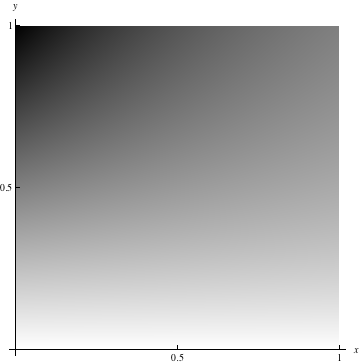
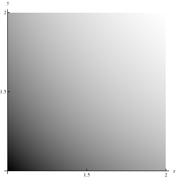
For reference, here are density plots from Problems 13.1 #7 and #21:

Density plot for Problem 13.1#7	Density plot for Problem 13.1#21

Tuesday, October 26

We are approaching integration within the context of computing total from density. Today, we worked out an example of computing total charge from an area charge density given for a flat rectangular region. In doing so, we saw our first example of a double integral and an iterated integral.

In Section 13.1, the authors approach double and iterated integrals within the context of computing volume for a solid region bounded by the graph of a function of two variables. This generalizes the idea of computing area for a planar region bounded by the graph of a function of one variable. In class, we will put more focus on the "total from density" interpretation/application because this context is relevant in other settings. The "area under a curve" or "volume under a surface" interpretation/application is not readily generalized to higher dimensions.

Exam #3 will be on Tuesday, November 2 from 9:30 to 10:50 am.

Here is the handout describing Project #2. The project is due on Friday, November 5. For reference, here is an earlier handout with general goals and requirements for projects.

We will not have class on Friday, October 29 to give those who are interested the opportunity to attend 2010 Race & Pedagogy National Conference events that will be taking place on campus.

Monday, October 25

Today, we turned our attention to the other half of caculus, namely integration. Fundamentally, integration is all about adding up infinitely many, infinitely small contributions to get a total. In generalizing the idea of definite integral to higher dimensions, we will often work with examples in which the goal is to compute a total amount of stuff given information about the density of the stuff. So, today we talked a bit about density. In particular, we discussed how a first view of density as density is mass divided by volume) needs to be generalized in three ways:

• other dimension: length, area, or volume
• other quantities: mass, number, charge, cost, probability,...
• uniform or non-uniform

We ended class with an example of computing total charge given information about the length density of a charge distribution. The problems on this handout will give you a bit more practice with this. Tomorrow, we will turn our attention to going from density to total in more than one dimension.

We will not have class on Friday, October 29 to give those who are interested the opportunity to attend 2010 Race & Pedagogy National Conference events that will be taking place on campus.

Friday, October 22

In class, we finished outlining the reasoning behind the second-derivative test. The two main pieces in this are

• understanding the nature of g(u,v)=Au²+2Buv+Cv² for various choices of A, B, and C; and
• using a Taylor series expansion to analyze f(x,y) for (x,y) near a critical point (x₀,y₀).

You can read the text's proof of the second-derivative test in Section 12.9. The authors have a different approach that uses some of the same elements we used in class. I am not assigning problems from Section 12.9.

We next turned our attention to approaches to constrained optimization problems. Problems 1, 2, and 4 on the applied optimization handout are examples of constrained optimization problems.

• The direct approach is to solve the constraint equation for one of the variables and to then substitute into the objective function. This reduces the number of variables in the objective function. We then analyze this reduced objective function to find the global minimum or maximum (whichever is of interest).
• The new approach is based on thinking about the constraint equation as giving a specific level curve for a constraint function. By looking at this level curve for the constraint function together with level curves for the objective function, we see that we want to find points at which the gradients of the two functions are parallel. If g is the constraint function and f is the objective function, this condition of parallel gradient vectors can be expressed as ∇f=λ∇g for some number λ.

The scaling factor λ is called a Lagrange multiplier and this new approach is called the method of Lagrange multipliers. In class, we set up an example but did not have time to finish solving the relevant system of equations. Here is a handout with the details of this example.

We will not have class on Friday, October 29 to give those who are interested the opportunity to attend 2010 Race & Pedagogy National Conference events that will be taking place on campus.

Thursday, October 21

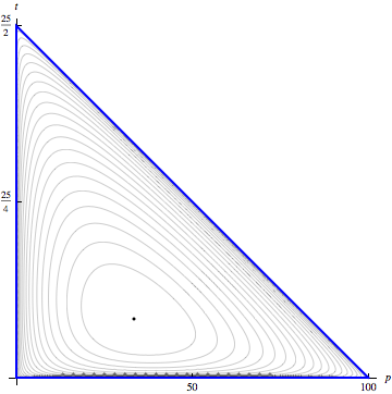
We spent a good part of class today working through most of the details of Problem 4 from the applied optimization handout. In the last part of this problem, we started analysis of the boundary of the relevent domain. In class, I set up the domain for this problem incorrectly. The correct domain is a triangle in the pt-plane, not the rectangle I had in class. The third side of the triangle is related to the constraint c=500-5p-40t. Negative values for c do not make sense in the context of the problem, so we need 0 ≤ 500-5p-40t. The third side of the triangle corresponds to equality in this so the equation of the line containing that third side is 0 = 500-5p-40t or p = 100-8t. Fortunately, analysis along this third side is easy since the utility function evaluates to 0 for all points on this segment.

The figure below shows the correct domain along with level curves for the utility function and the critical point we found at p=100/3, t=25/12. The maximum utility occurs at this critical point.

After looking at questions on homework problems, we turned our attention to providing some explanation of the second-derivative test for classifying critical points. We'll finish that discussion tomorrow.

Friday, October 15

In class, you worked out the details of a global extreme values example and then started on the first problem from the handout with applied optimization problems.

The assignment for Section 12.7 originally had a problem to be submitted on Thursday, October 21. I've changed the due date for this to Friday, October 22. Note that I have also added a problem to be submitted from the applied optimization handout.

Have a great break!

Thursday, October 14

In class, we looked at local extreme values and global extreme values. For both, we want to distinguish between what it is and how to find it.

"What it is" for local extreme values is given by the following definition.

Definition: Given a function f:R²→R, we say an input (x₀,y₀) is a local maximizer and the corresponding output f(x₀,y₀) is a local maximum if there is an open disk centered at (x₀,y₀) such that f(x₀,y₀) ≥ f(x,y) for all (x,y) in that disk. Local minimizer and local minimum are defined similarly with the inequality reversed.

"How to find it" for local extreme values generally consists of two steps:

1. Find all critical points by solving the system of equations given by setting the two first-partial derivatives equal to zero.
2. Analyze each critical point to classify it as a local minimizer, a local maximizer, or neither. For this, use either direct analysis or the second-derivative test.

"What it is" for global extreme values is given by the following definition.

Definition: Given a function f:R²→R and a domain D, we say an input (x₀,y₀) is a global maximizer and the corresponding output f(x₀,y₀) is the global maximum if f(x₀,y₀) ≥ f(x,y) for all (x,y) in D. Global minimizer and global minimum are defined similarly with the inequality reversed.

"How to find it" for global extreme values generally consists of three steps:

1. Find all critical points in D by solving the system of equations given by setting the two first-partial derivatives equal to zero. Compute the output for each critical point.
2. Analzye the function along the boundary of D. Often this consists of breaking the boundary into pieces and analyzing a function of one variable along each piece to find "boundary critical points" and endpoints. Compute the output for each of the relevant input points found along the boundary.
3. Look through the list of computed outputs to pick off the global minimum and global maximum. Note that there will be at most one global minimum value and at most one global maximum value but each may occur at more than one input.

Project #1 is tomorrow. Come talk with me if you have questions on your work or writing.

Tuesday, October 12

After addressing questions from the handout on differentials and some comments on a few problems from Exam #2, we had a few minutes to start thinking about extreme values. As with many things we do in this course, we will be generalizing ideas from calculus for functions of one variable. For functions of one variable, the story of extreme values starts with a definition: Given a function f:R→R, we say an input x₀ is a local maximizer and the corresponding output f(x₀) is a local maximum if there is an open interval I centered at x₀ such that f(x₀) ≥ f(x) for all x in I. This tells us what a local maximum is. The next part of the story is to ask "How do we fina local maxima?" As you know, one approach is to look for inputs for which the derivative f′(x) is zero. Our generalization of this story to functions of two or more variables will seem very natural in many ways. We'll pick up this story on Thursday.

Project #1 is due on Friday. Come talk with me if you have questions on your work or writing.

Monday, October 11

In class, we looked at how to use differentials to relate small changes among variables. Generally, we start with a nonlinear relation among various variables and we then compute a linear relation among the differentials for those variables. Differentials can be thought of as coordinates in the "zoomed-in world". Differentials are always related linearly. Ratios of differentials give rates of change. No limit is needed since the limit process has already been taken care of in "zooming in" process.

Working with differentials complements working with the linearization function L. Differentials are useful when we want to focus on change and rate of change. Linearizations are useful when we want to focus on approximating specific output values.

Project #1 is due on Friday. Come talk with me if you have questions on your work or writing.

Friday, October 8

In class, we reviewed linearization and tangent lines for functions of one variable and then considered linearization and tangent planes for functions of two variables. The linearization of a function f is a linear function L built using information about f at a specific point (x₀,y₀). If the function is differentiable at a point, then the linearization based at that point is the best linear approximation. One subtlety for functions of two (or more) variables is that the linearization might exist even if the function is not differentiable. For the linearization to exist, it is enough to have the two first partial derivatives exist. As we saw in an example yesterday, existence of the first partial derivatives is, alone, not enough to guarantee differentiability.

The text's approach to tangent planes and linearization for functions of two variables differs from what we did in class. The text starts with the more general idea of a tangent plane to a surface at a point where that surface is not necessarily the graph of a function z=f(x,y). In reading Section 12.6, you can focus on

• Example 2 on page 749 and the box just above that example
• The subsection "How to linearize a function of two variables" on pages 751-752
• The subsection "Functions of more than two variables"

You should also read the subsection "Differentiability" on pages 727-728 and think about how this connects to ideas we saw in class today.

On Monday, we will talk about differentials. This will provide us with a clean and powerful way to look at the linear relations that underlie linearization.

In class, we did not finish off an example of getting an upper bound on the error in a linear approximation for a function of two variables. I've written up the details in this handout.

Thursday, October 7

I returned Project #1 drafts today along with these comments on some finer points of style. The final version will be due on Friday October 15. As we discussed in class, a well written paper that uses specific parameter values to find and analyze one non-ideal gas law behavior will earn a grade in the B+/A- range. A well written paper that goes beyond this will push into the A range. Examples of going beyond include

• finding and analyzing more than one type of non-ideal gas law behavior, and/or
• working with unspecified values of the parameters to deduce general features or details of level curves.

In this case, a full understanding of level curves in the relevant domain (V>nb, p>0) will reveal three distinct types of level curve (or four depending on how you count, but really just three) and two special level curves separating those regions.

In class, we discussed some technical details from Section 12.3 that we had not previously looked at carefully. One set of deatails concerns the hypotheses that guarantee equality of mixed partial derivatives. The other set of details concerns a definition of differentibility for functions of several variables and the hypotheses on partial derivatives that guarantee a function is differentiable at a given point.

As homework, you should read the theorems and definitions on pages 726-728 of the text. The context of Theorem 3 and the wording of the definition of differentiable may initially be a bit mysterious. We'll get some insight on these tomorrow as we talk about tangent planes.

I am not assigning homework problems related to the ideas we discussed in class. For an optional challenge, you can work out the details of the example we saw of a function that does not have equality of mixed partial derivatives. (Exercise 1 on page 783 in the Additional and Advanced Exercises section is statement of this problem.)

Tuesday, October 5

Monday, October 4

Exam #2 will be tomorrow, Tuesday, October 5. We will use the 80 minute period from 9:30 to 10:50. It will cover material from Sections 12.1 through 12.5. This handout has a list of specific objectives for the exam.

I have reserved TH 381 starting at 7 pm this evening for a Math 280 study session. If you are looking for others to study with, come to TH 381 after 7 pm and find a small group working on something of interest.

Friday, October 1

In class, we did three things:

• reviewed the definition of gradient vector that we set up yesterday,
• determined how to compute the components of a gradient vector, and
• determined how to use a gradient vector to compute a directional derivative

While the reasoning we went through to connect these three things may initially be challenging, the take-away messages are simple:

• The gradient at each point is a vector \(\vec\nabla f\)
  • that points in the direction of greatest rate of change, and
  • has magnitude equal to that greatest rate of change.
• In cartesian coordinates, components of gradient vectors are computed as \(\displaystyle \vec\nabla f=\frac{\partial f}{\partial x}\hat{\imath}+ \frac{\partial f}{\partial y}\hat{\jmath}. \)
• The directional derivative in the direction of the unit vector \(\hat{u}\) is given by \(\displaystyle \frac{df}{ds}=\vec\nabla f\cdot\hat{u}. \)

Here's a handout outlined the reasoning we discussed in class. A key part of this reasoning is that infinitesimal changes \(df\) in outputs are related to infinitesimal displacements \(d\vec{r}\) by \( df=\vec\nabla f\cdot d\vec{r}\).

Note: In class, we denoted a directional derivative by \(df/ds\). The text uses a different notation, namely \(D_{\hat{u}}f\).

Exam #2 will be on Tuesday, October 5. We will use the 80 minute period from 9:30 to 10:50. It will cover material from Sections 12.1 through 12.5. This handout has a list of specific objectives for the exam.

Thursday, September 30

In class, we started in on the last set of ideas before the exam by working through this handout on estimating greatest rate of change for a function of two variables. Since greatest rate of change involves both direction and magnitude, we represent the greatest rate of change as a vector at each point in the domain of the function. These are called gradient vectors. So, at each point in the domain of the function, a gradient vector

• points in the direction of greatest rate of change
• has magnitude equal to that greatest rate of change.

Tomorrow, we will see how to compute components of gradient vectors using partial derivatives. We will also see how to use a gradient vector to compute a directional derivative to get the rate of change in a specified direction.

A draft of Project #1 is due on Friday, October 1.

Exam #2 will be on Tuesday, October 5. We will use the 80 minute period from 9:30 to 10:50.

Tuesday, September 28

In class, we looked at some examples of chain rules involving partial derivatives. Chain rules are relevant when differentiating functions that are compositions of other functions. In the context of functions of more than one variable, there are many ways to build compositions so there are many chain rules. Rather than trying to memorize a chain rule for each specific type of composition, you should work to understand how the pieces of a chain rule fit together in general. Tree diagrams are one way of doing this.

A draft of Project #1 is due on Friday, October 1.

Exam #2 will be on Tuesday, October 5.

Monday, September 27

The main goal for class today was to start becoming proficient with the mechanics of computing partial derivatives. I've assigned (a lot) of problems from Section 12.3 so that you can master these mechanics. You'll need to recall all of your differentiation techniques from first-semester calculus and you'll need to keep the right mindset.

A draft of Project #1 is due on Friday, October 1.

Exam #2 will be on Tuesday, October 5.

Friday, September 24

Today, we started our look at differentiation in the context of functions of several variables by thinking about rate of change for a specific example, namely the relationship between T, p, and V given by the ideal gas law. On the worksheet, you used a plot of level curves for T in the Vp-plane to estimate

• rate of change in T with respect to V, and
• rate of change in T with respect to p

for a variety of points. We can use derivatives to get exact values rather than estimates. We'll look at the details of differentiation in the context of functions of several variables starting Monday.

We've just gotten a first look at the ideas in Section 12.3 without enough detail for you to work on problems from that section. So, for now, you should finish off the worksheet we started in class and you should have a quick read of Section 12.3. You can also be working on Project #1.

If you are interested in the details, here is the entry in a New York Times series on drawing featuring ellipes that we looked at briefly in class.

Thursday, September 23

In class, we looked at a precise definition of limit for functions of two variables and at some of the facts about limits that follow from this definition. For reference, here's the two versions of the definition that we saw:

• \(L\) is the limit of \(f\) for \((x_0,y_0)\) if for every target interval centered at \(L\) there is a launch disk centered at \((x_0,y_0)\) so that every \((x,y)\) in the launch disk has \(f(x,y)\) in the target interval.
• \(L\) is the limit of \(f\) for \((x_0,y_0)\) if for every value of \(\varepsilon>0\) there is a value of \(\delta>0\) so that \(\sqrt{(x-x_0)^2+(y-y_0)^2}<\delta\) implies \(|f(x,y)-L|<\varepsilon\).

These two statements say the same thing in different ways. The second statement has the advantage of being easy to generalize to functions of three or more variables. In this course, we will not spend enough time to master this precise definition. Instead, we will accept some basic facts that follow from this definition so that we can efficiently evaluate many limits.

You should now be working on assigned problems from Section 12.2 using the ideas and examples we discussed in class. We'll address questions from these in class tomorrow.

Tuesday, September 21

One goal for today was to form a "big picture" of how continuity and discontinuities generalize in going from functions of one variable to functions of two or more variables. The notion of continuity as "graph is an unbroken curve" is not readily generalized so we need to rely on a more carefully phrased definition. That definition is essentially "limit at input exists and is equal to the given output." This definition can be applied to functions of more than one variable. To do so, we first need to think about what limits mean for functions of more than one variable. We'll discuss this on Thursday. In the meantime, I've assigned problems from Section 12.2. You should see how much progress you can make on these by applying what you know about limits for functions of one variable.

One of you has noticed that the tentative schedule I distributed on the first day of class lists a due date on Thursday for a draft of the first project. I am moving this due date back until at least next week. I'll distribute details about the first project in class on Thursday.

Monday, September 20

In anticipation of ideas to come, we thought briefly about the structure of level curves for a function of two variables if we zoom in on a point. With sufficient zooming, we should see level curves as a stack of parallel lines. At each point, the stack will have a particular orientation and a particular density (for equal-sized changes in the output variable). We'll soon come to see this information represented as a vector (at each point). This vector is one notion of derivative for functions of two variables.

Visualizing functions of three variables presents challenges since we need three dimensions to represent inputs and a fourth dimension for the output axis. The graph of a function of three variables is a three-dimensional object sitting in four dimensional space. We won't visualize this directly. Instead, we will limit ourselves to visualizing contours (a.k.a. level surfaces). Level surfaces are natural generalizations of level curves for functions of two variables. You can play with an example of some level surfaces for a particular function here.

In mnay cases, we will not take time to visualize level surfaces in detail, but will want to keep a generic picture in mind of a set of nested surfaces. We can generalize the idea we started with by thinking about zooming in on a point. With sufficient zooming, we should see level surfaces as a stack of parallel planes. At each point, the stack will have a particular orientation and a particular density (for equal-sized changes in the output variable). A vector can be used to encode this information.

I've assigned a few additional problems from Section 12.1, including one to be submitted on Thursday.

If there are things you do not understand from the material covered by Exam #1, come talk with me as soon as possible so we can solidify those ideas for you.

Friday, September 17

Our next focus in the course will be functions of several variables. We started today by looking at examples of functions of two variables. The usual ideas of function are relevant: domain, range, and graph. Building or visualizing a graph requires thinking in three dimensions since we need two coordinates for the inputs (x,y) and one coordinate for the output z=f(x,y). One approach to is to sketch contours in the input plane. A contour in the input plane is a curve along which the output has a constant value.

I've assigned a few problems from Section 12.1 that involve thinking about functions of two variables. After Monday's class, I'll assign some additional problems including one or two to submit.

Once we get some comfort with the basics of functions of several variables, we'll turn our attention to calculus concepts (limit, continuity, differentiation, integration) in this new context.

Note that we will be skipping over one last idea from Chapter 10 (namely, cross products) and all of Chapter 11 for now. We'll come back to this material later in the semester.

In class, I have been using the mathematical computing program Mathematica to help visualize some of the surfaces we've been looking at. You can also get to some of Mathematica's capabilities online through the Wolfram Alpha web site. (Wolfram is the company that produces Mathematica. Wolfram Alpha is a web-based service to provide information and do computations.)

Thursday, September 16

Tuesday, September 14

Exam #1 will be on Thursday September 16. We will use the 80 minute period from 8:00 to 9:20. The exam will cover material from Sections 9.4, 10.1, 10,2, 10.3, 10.6 and the two handouts on equations of planes. This handout has a list of specific objectives for the exam.

I will be available for office hour today (Tuesday) from 12:30 to 1:30 and for appointments after that until 4:00. On Wednesday, I will be available most of the day except noon to 2:00 pm. If you have questions, email or call to set up a time to talk. I can also try to address questions sent by email, although using mathematical notation is not always possible.

Monday, September 13

In class, we talked about two ideas that involve the dot product. One is the idea of computing the component and projection of one vector in the direction of another vector. These two things are closely related. The component of one vector in the direction of another is a number; the projection of one vector in the direction of another is a vector. The dot product is useful in computing both of these.

The other idea we discussed in class is what we will call the point-normal form for the equation of a line. The starting point for this equation is to consider specifying a plane by giving a point on the plane and a vector perpendicular to the plane. Such a vector is called a normal vector. There are details on this in Section 10.5 but these are mixed in with several other ideas so I have pulled out the main idea we want on this handout.

Exam #1 will be on Thursday September 16. We will use the 80 minute period from 9:30 to 10:50. The exam will cover material from Sections 9.4, 10.1, 10,2, 10.3, 10.6 and the two handouts on equations of planes. This handout has a list of specific objectives for the exam.

If you are interested in using the mathematical computing program Mathematica that I have occasionally used in class, you can find it on many computers on campus. (It is definitely on the computers in the Thompson Hall computer lab.) There is a small glitch in the installation of the software that points to an invalid address for something called the license server so you might get an error message if you are the first person to launch Mathematica on any particular machine. If so, you will get a dialog box with a warning about failing to connect to a license server. To fix things, press the Enter Password button in this dialog box. This will bring up a new dialog box with two options: "Single Machine License" or "Network License". Choose the "Network License" option and then enter the server name "errol.pugetsound.edu" in the box provided. That should do it. This will only need to be done once on each machine so you won't need to do it again if you return to the same computer.

Friday, September 10

Today, we introduced the idea of dot product. This is an operation that takes two vectors and results in a number. In terms of components, the dot product is given by \[\vec{u}\cdot\vec{v}=u_x v_x+u_y v_y+u_z v_z.\] In terms of geometry, the dot product is given by \[ \vec{u}\cdot\vec{v}=\|\vec{u}\|\,\|\vec{v}\|\cos\theta\] where \(\theta\) is the angle between the two vectors. In many situations, you will want to think geometrically (using the second expression) and then compute in terms of components (using the first expression).

I have assigned problems from Section 10.3 that deal with dot product. Note that you can leave parts (c) and (d) of #1-7 odd along with 21 and 23 until after class on Monday. Those problems will make more sense after we discuss some additional details about dot products in class.

One of you has pointed out that for Section 10.6 #43, the picture in the answer section of the text is not accurate (if we assume that the length scales for all three axes are the same). The cross-section in the yz-plane is an ellipse with its major axis along the z-axis and its minor axis along the y-axis. The picture in the answer section shows an ellipse with a different orientation. To get the correct picture, the entire surface should be rotated by 90 degrees around the x-axis.

For Section 10.2 Problem 49(c), you can take advantage of the fact that the medians of a triangle all intersect at a point that is two-thirds of the way along each median (starting from a vertex). So, to get from the origin O to the median intersection point Q, you can go from the origin to the point C and then two-thirds of the way down the median starting at C. Using vector addition, we can write this as \[ \overrightarrow{OQ}=\overrightarrow{OC}+\frac{2}{3}\overrightarrow{CM}.\] The components of the vector \(\overrightarrow{OQ}\) will give you the coordinates of the point Q.

Exam #1 will be on Thursday September 16. If possible, we will use the 80 minute period from 9:30 to 10:50. If you have not already replied to my email asking whether or not this works for your schedule, please do so as soon as possible.

Thursday, September 9

In class, we continued developing basic ideas about vectors. As you begin to master (or review) these ideas, try to develop both geometric and algebraic ways of working with vectors. In many contexts, you will find it useful to get started by geometrically and then turn to components to compute.

Exam #1 will be on Thursday September 16. If possible, we will use the 80 minute period from 9:30 to 10:50. If you have not already replied to my email asking whether or not this works for your schedule, please do so as soon as possible.

Tuesday, September 7

Today, we began talking about vectors. Since we've just gotten started on this, I've only assigned a few problems from Section 10.2. I'll assign more after Thursday's class.

If you are interested, you can read more about the use of geometry in Gaudi's design of the Sagrada Familia cathedral in Barcelona.

I've added more plots of quadric surfaces to the Math 280 3D Picture Gallery. For another view of quadric surfaces, you can go to the Interactive Gallery of Quadric Surfaces developed by Jonathon Rogness at the University of Minnesota. The plots in this gallery allow you to manipulate the cross-sections of the quadric surfaces. (Professor Rogness is also one of the creators of a cool short film called Mobius Transformations Revealed.)

Friday, September 3

Our focus in class today was quadric surfaces. There is a brief catalog of these on page 655 of the text. We looked at a few examples in class. Rather than trying to memorize the catalog on page 655, it is more important to master the ability to look at cross-sections and then see how those fit into a surface.

You can view some interactive three-dimensional pictures (similar to ones we looked at it class) at the Math 280 3D Picture Gallery. I'll be adding more examples to this over the next few days.

Enjoy the long weekend.

Thursday, September 2

In class, we reviewed some basics of ellipses, parabolas, and hyperbolas. In particular, we started from a purely geometric definition for each type of curve and then introduced a coordinate system to get an analytic description. In all three cases, the analytic description is a quadratic equation in two variables.

We can also turn this around and ask about the graph of any quadratic equation in two variables. It is a fact that the graph of any quadratic equation in two variables is an ellipse, a parabola, or a hyperbola. That is, the graph of any equation of the form

\[ Ax^2+2Bxy+Cy^2+Dx+Ey+F=0\qquad A,B,C\textrm{ not all zero} \]

is an ellipse, a parabola, or a hyperbola. You can determine which type of curve by computing \(AC-B^2\). If this quantity is positive, the graph is an ellipse. If this quantity is zero, the graph is a parabola. If this quantity is negative, the graph is a hyperbola.

Tomorrow, we will bump these ideas up to three-dimensions so we will be dealing with quadratic equations in three variables and the corresponding graphs that are surfaces in space.

Tuesday, August 31

In class, we looked at equations of planes. In the text, this material is covered in Section 10.5 using some ideas we have not yet developed. We will soon get to those ideas, but for now you can use this handout on equations of planes. All of the ideas here are natural generalizations of equations of lines in a plane.

Monday, August 30

In class, we began exploring three-dimensional space using cartesian coordinates. We first looked at the graph of a function of two variables, specifically z=x³y², and then as some simpler geometric objects (such as planes). You should start working on the assigned problems from Section 10.1. As part of this, you will need to read Section 10.1 about equations of spheres in space. This is a straightforward generalization of equations of circles in a plane.

Here is an interactive plot of the function graph we looked at in class. You can rotate and zoom to look at this from various perspectives.

To get some sense of what is expected in terms of the prerequisite courses in the calculus sequence, you might find it useful to look at this Math 180 final exam and at this Math 181 final exam from the most recent times I have taught each of these courses.

Handouts

• Math 180 final exam (Monday, August 30)
• Math 181 final exam (Monday, August 30)
• Equations of planes (Tuesday, August 31)
• Equations of planes 2 (Monday, September 13)
• Estimating rate of change (Friday, September 24)
• Partial derivatives practice (Monday, September 27)
• Estimating greatest rate of change (Thursday, September 30)
• Components of the gradient vector (Friday, October 1)
• A linearization example (Friday, October 8)
• Problems on differentials (Monday, October 11)
• Applied optimization problems (Friday, October 15)
• Lagrange multiplier example (Friday, October 22)
• Problems: Total from length density (Monday, October 25)
• Three solutions to Section 12.8 #10 (Friday, October 29)
• Problems: Total from area density (Monday, November 1)
• An example of evaluating a double integral using polar coordinates (Friday, November 5)
• Problems: Total from volume density (Monday, November 8)
• Using the Greek alphabet in mathematics (Tuesday, November 9)
• The volume element in spherical coordinates (Friday, November 12)
• Exam #4 objectives (Monday, November 15)
• Big picture view of integration (Friday, November 19)
• Integration over a curve (Friday, November 19)
• Problems: Integration over a curve (Friday, November 19)
• Integration over a surface (Monday, November 29)
• Problems: Integration over a surface (Monday, November 29)
• Integrating a vector field over a curve (Friday, December 3)
• Conservative vector fields (Tuesday, December 7)
• Exam #5 topics and text (Tuesday, December 7)

Projects

• Overview of projects
• Project #1 First draft due Friday, October 1; final version due Friday, October 15
• Comments of Project #1 drafts
• Project #2 Due Tuesday, November 9 (originally Friday, November 5)
• Project #3 Due Monday, December 6

Exam objectives

• Exam #1 objectives
• Exam #2 objectives
• Exam #3 objectives
• Exam #4 objectives
• Exam #5 objectives

Old exams

You can look at exams from last time I taught Math 280. You can use these to get some idea of how I write exams. You can use these old exams to prepare for our exams in whatever way you want. I will not provide solutions for the old exam problems but you are welcome to discuss these problems with me.

Don't assume I am going to write our exams by just making small changes to the old exams. Also note that there may be differences in order and emphasis of topics between these exams and our course.

Useful Class Links

• TI calculator support (including downloadable manuals)

Fun Stuff

• The Mathematical Atlas describes the many fields and subfields of mathematics. The site has numerous links to other interesting and useful sites about mathematics.
• If you are interested in the history of mathematics, a good place to start is the History of Mathematics page at the University of St. Andrews, Scotland.
• For a history of some mathematical terminology, see Earliest Known Uses of Some of the Words of Mathematics.
• For a similar history of some mathematical symbols, see Earliest Uses of Various Mathematical Symbols.
• Check out the Astronomy Picture of the Day.
• Read about some of the geometric ideas in the architecture of the Sagrada Familia cathedral in Barcelona.