Math 280

Multivariate Calculus

Spring 2007

Homework assignments

Daily notes

Monday, May 7

I realized today that the version of the Fall 2006 final exam I had posted at the beginning of the semester was, in fact, a draft. For reference, here's links to the draft and the final version:

• Draft of Fall 2006 final exam
• Final version of Fall 2006 final exam

Note that the draft has many more questions than the final version. The draft also has a few typos. One of you pointed out these to me:

• In Problem 3, the point should be (0,2,5π/2) rather than (0,2,10π).
• In Problem 9, the formula should read δ=kρsin(θ/2) rather than δ=krsin(θ/2)

Wednesday, May 2

In class, I distributed this handout with some notes on logisitics and the final exam. As an additional source of problems, here's the final exam from my Spring 2004 section of multivariate calculus.

Tuesday, May 1

Monday, April 30

Friday, April 27

Exam #5 will be on Tuesday, May 1 from 9:30-10:50. It will focus on material we have covered since the previous exam. This is most of Chapter 14. This handout has a list of sections from the text in the order we have covered them in class. For your reference, here's Exam #5 from my Spring 2004 section of multivariate calculus. This exam better reflects what to expect for our Exam #5 than anything from the Fall 2006 course.

Wednesday, April 25

In class today, we looked at the operator view of divergence and curl. One advantage of this view is that it can help us remember how to compute the curl of a vector field, provided we remember how to compute the cross product.

I've assigned a few problems from Section 14.8 that deal with proving various identities. An example of this is given in Equation (8) on page 911. The basic plan for proving one of these identities is to express everything in terms of components. You'll then be able to use various properties of partial derivatives (such as sum and product rules).

At the end of class, I described an interpretation of divergence and curl in terms of thinking about the vector field as giving velocity of a fluid flow. At each point A in space, we have three things to consider:

• the output F(A), which is a vector
• the divergence of F, which is a scalar
• the curl of F, which is another vector

To interpret divergence, consider placing a small drop of dye that moves with the flow into the fluid. Watch this dye drop as it moves with the flow through the point A. The divergence divF(A) gives the rate of change in the volume of the dye drop with respect to time. So, a positive value of divF(A) means the volume of the dye drop increases as the it moves through the point A and a negative value of divF(A) means the volume of the dye drop increases as the it moves through the point A.

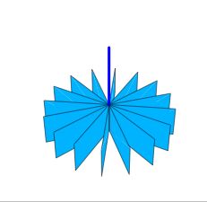
Interpreting curl is a bit more complicated since curl F(A) is a vector. In class, we talked about putting a pinwheel in the fluid flow at the point A. This is not really the right image. The blades of a pinwheel are shaped so that the pinwheel spins fastest when the pinwheel is oriented to face the fluid flow "head-on". Rather than a pinwheel, we really want to consider a paddlewheel. Think of this like the paddlewheel on the kind of boat that goes up and the Mississippi. The blades of the paddlewheel are parallel to the central axis. Here's what you might picture:

• If we orient the axis of the paddlewheel parallel to the x-axis, then p=i. The dot product i·curl F(A) is equal to the i-component of curl F(A). So, the i-component of the curl tells us how fast the paddlewheel rotates when its axis is parallel to the x-axis. A similar story holds for the j and k components of curl.
• To get the greatest rotation speed, we would orient the paddlewheel so that p is parallel to curl F(A) itself. This follows from the fact that the dot product of two vectors of fixed magnitude is largest when the vectors have the same direction.
• That greatest rotation rate is proportional to the magnitude of curl F(A). This follows from the geometric view of dot product:
  p·curl F(A) =|p| |curl F(A)|cos0 =(1)|curl F(A)|(1) =|curl F(A)|.

Tuesday, April 24

I've assigned problems from Section 14.6 that involve evaluating surface integrals for vectors fields. For each problem, choose the approach that seems best:

• thinking geometrically
• using an implicit description of the surface
• using a parametric description of the surface

In class, I have focussed on the first two approaches. This handout has another example of evaluating a surface integral using an implicit description of the surface. The text focusses on using a parametric description.

The text introduces another approach to evaluating surface integrals (or either a scalar function or a vector field) that is based on viewing the surface S as part of a level surface for a function of three variables and then using the fact that the gradient of that function is normal to the level surface. Formula (3) on page 897 and Formula (6) on page 900 use this idea. You are welcome to understand this idea but I will not require you to use it.

In class, I threatened to assign some problems from Sections 14.7 and 14.8 that involve computing divergence and curl of vector fields. Instead, I've put together a handout with a few problems.

Monday, April 23

I haven't yet assigned problems from Section 14.6 on surface integrals for vector fields. I'll do this after tomorrow's class.

Friday, April 20

I've assigned problems from Section 14.3. Most of the problems use notation that we haven't used a lot in class. This notation is the last one given in Table 14.2 on page 861. In this notation, the integrand of a line integral is expressed as M dx+N dy+P dz. This is equivalent to F·dr To make the connection, write F=M i+N j+P k and dr=dx i+dy j+dz k. Using these component expressions to compute the dot product, we have F·dr=M dx+N dy+P dz. Turning this around, given M dx+N dy+P dz, we can read off the components of F to get F=M i+N j+P k

All of the problems I have assigned from Section 14.3 amount to asking whether or not a given vector field has a potential function or to using the FTC for Line Integrals to evaluate a given line integrals. For historic reasons, there are many different ways to say the same thing in this material. All of the following phrases are essentially equivalent:

• F has a potential function
• F is conservative
• the line integral of F is path-independent
• M dx+N dy+P dz is exact

We'll look at these in a bit more detail on Monday (and give some conditions to make precise the claim that these are essentially equivalent).

In case you are bored and looking for something to read this weekend, I'm posting this handout on line integrals. The handout has three parts: definition of line integral, a note on notation (expanding a bit on what's above), and an example of evaluating a line integral using two different methods. There's nothing really new here so you don't need to look at this.

Wednesday, April 18

I've assigned additional problems from Section 14.2 that involve line integrals for vector fields.

Tuesday, April 17

In class, we began talking about vector fields. I drew two examples of planar vector fields (i.e., vector fields in the plane). I also described some vector fields in space. Here are 3D versions of two examples that you can rotate to view from different angles.

You can use computing technology to make vector field plots. One nice tool for plotting (and analyzing) a vector field plot is the Vector Field Analyzer (written by Matthias Kawski of the Mathematics Department at Arizona State University ). This Java applet allows you to plot and analyze a two-dimensional vector field. Be patient as the page loads; it takes a minute or two for the Java code to set everything up. After the code is loaded, you will see a plot of the default vector field. To plot a different vector field, enter the components of the vector field you want in the boxes near the bottom of the applet window and then click on the button "Plot this field." You should try the simple examples we have looked at in class such as F=x i+y j and F=-y i+ x j . The Vector Field Analyzer has lots of features (and a few bugs).

One feature you should play with is based on thinking of vector field outputs as velocity vectors for fluid flow. Click on the tab labeled "DEs/flows." This part of the program lets you draw a box on the vector field plot and then watch as the box "goes with the flow."

I've posted some problems from Section 14.2 that deal with vector fields. Tomorrow, we will look at line integrals for vector fields. I'll then post more problems from Section 14.2

Monday, April 16

To evaluate a surface integral, our basic strategy is to set-up an equivalent iterated integral in two variables and then to evaluate that iterated integral. One way or another, we need to pick two variables in which we can express the integrand, the area element, and limits of integration. The text focusses on parametrizing the surface with a vector-output function of two variables. In class, we've looked at other approaches. This can include direct geometric reasoning or working with an implicit description of the surface.

In class today, we computed the surface area of a sphere by expressing the area element in terms of cartesian coordinates for the projection of the sphere into a plane. Here's a 3D version of the picture for this I drew in class that you can rotate to view from different angles. If I have time later, I'll put up versions showing pictures relevant to the method we used last Friday and to the polar coordinates we used today.

I've assigned problems from Sections 14.5 and 14.6. Start each problem by thinking about what approach is most natural or will be easiest to carry out. Note that the problems for Section 14.5 all involve computing total surface area so the integrand is 1. For the surface integrals in Section 14.6, the integrand is not necessarily 1.

Friday, April 13

We will approach the material of Chapter 14 in an order that differs from the text in places. Today, we talked about surface integrals for scalar-output functions. This material is covered in Section 14.5 and the first part of Section 14.6 in the text.

In class, we did one example of computing a surface integral (to get surface area). This example involved a sphere so we were able to get a coordinate expression for dA using geometric reasoning. For other surfaces, we'll need to work a bit harder to get an expression for dA. One approach is to parametrize the surface. I've assigned problems from Section 14.5. Focus on the first four which involve parametrizing surfaces but not computing surface integrals.

Wednesday, April 11

The text approaches the evaluation of a line integral by parametrizing the curve with a vector-output function r(t). For the example we worked on in class, this was the third method that we didn't get to. I've written a handout with details on what we did in class and the details of the third method we did not have time to cover. Example 3 on page 854 of the text is similar to what we did in class, although the density function is different. (Note that the text uses the symbol δ for density without distinguishing among length, area, and volume densities.)

Tuesday, April 10

Monday, April 9

Exam #4 will be tomorrow (Tuesday, April 10) from 9:30-10:50. It will focus on material from Sections 13.1 through 13.7.

I will have office hour this evening from 7:00-8:00 pm at the north end of the third floor of Harned Hall.

Friday, April 6

Wednesday, April 4

Exam #4 will be on Tuesday, April 10 from 9:30-10:50. It will focus on material we will have covered since the previous exam.

Note that there are different conventions for naming and ordering spherical coordinates. For reference, let's describe these in relation to a cartesian coordinate system. In class, we are using

• ρ for the radial distance from the origin to the point P
• ϕ for the angle measured from the positive z-axis to the ray from the origin through P
• θ for the angle measured from the positive x-axis to the ray from the origin though the point Q that is the projection of P onto the xy-plane.

We list this in the order (ρ, ϕ, θ). The text (and most U.S. math texts) labels the coordinates with the same variables but lists them in the order (ρ, θ, ϕ). Most physics texts use r for the radial coordinate, θ for the angle measured from the positive z-axis and ϕ for the other angle, listing these in the order (r, θ, ϕ).

Tuesday, April 3

If you understand polar coodinates (r,θ) for the plane, then you should be in good position to understand cylindrical coordinates for space. Cylindrical coordinates amount to using polar coordinates together (r,θ) with the cartesian coordinate z to get coordinates (r,θ,z) for points in space. For iterated integrals in cylindrical coordinates, the appropriate form of the volume element is dV=r dr dθ dz.

We are now using triple integrals to get the total of some quantity given a region of space and the volume density for that quantity. (The quantity might be mass, charge, cost, or probability.) In class, I use the Greek letter ρ ("rho") for volume density. Recall that we have used λ ("lambda") for length density and σ ("sigma") for area density. The textbook uses δ ("delta") for length, area, or volume density.

Carl asked about multiple integrals in dimensions higher than three. One application that can involve high dimensions is computing a total joint probabilityfrom a joint probability density function for two or more continous random variables. My example in class for this wasn't very good or clear. This link gives a better and more detailed example for two continous random variables. This example is related to queuing theory which is used to choose good ways to set up waiting lines (or queues). The queues might be for people (as at Disneyland) or for information flow in a computer or for parts in a factory or... Queuing theory is part of a field called operations research. Operations research is about using quantitative methods to make good decisions. You can learn more about it at the INFORMS web site.

Monday, April 2

When we looked at Problem 19 from Section 13.4 in class today, some people expressed discomfort with the fact that we used -π/6 to π as the range of θ values to describe a particular petal of the rose given by the polar equation r=12cos 3θ. The beginning value and end value of θ that define a petal are given by the condition r=0 so you can look at the solutions of the equation cos 3θ=0. This equation has infinitely many solutions so you'll still want to have a plot of the curve to help decide which solutions are relevant.

Sections 13.5 and 13.6 concern integrals and iterated integrals in three variables. I am going to turn you loose on problems from Sections 13.5 and 13.6 (or turn the problems loose on you, depending on how you look at it) without having spent more than 30 seconds of class time on triple integrals and iterated integrals in three cartesian coordinates. These ideas are natural extensions of double integrals and iterated integrals in two cartesian coordinates. You can handle this.

Section 13.6 includes material on computing total mass from a given volume density function. There is also material on center of mass and moments of interia. We will not focus on these last two topics. If you are taking physics, or plan to do so, you should look at the material on the last two topics. You can come talk with me outside of class if you have questions on it.

Friday, March 30

We hit polar coordinates quickly in class today because some people have more experience with them than others. If things in class are moving too quickly for you, come see me outside of class early next week. Here's the main ideas of polar coordinates we will use:

• plotting points in polar coordinates
• plotting polar curves
• describing planar regions with bounds on polar coordinates
• transforming between cartesian and polar coordinates

You can use Section 9.1 of our text as a reference on polar coordinates. Do some problems from this section if you need some practice.

Our main use of polar coordinates will be in evaluating a double integral by setting up an equivalent iterated integral in polar coordinates and then evaluating that iterated integral. The main elements in setting up an iterated integral in polar coordinates are

• describing the region of integration with appropriate bounds on polar coordinates
• expressing the integrand in polar coordinates
• using dA=r dr dθ for the area element

When you are describing the region of integration in polar coordinates, it is often best to start by finding the angular wedge that just contains the region. This gives you a lower bound and an upper bound on the polar angle θ. Then, think about going across the region in the radial direction (i.e., directly away from the origin) for various angles in this wedge. For each angle, identify the lower bound on r and the upper bound on r. One or both of these may depend on θ. Make sure the dependence is the same for the entire wedge. Otherwise, break the wedge into two or more smaller wedges and find lower and upper bounds on r for each wedge.

For many of the problems from Section 13.4, you will be given an integrand in cartesian coordinates. You can convert this to polar coordinates using the tranformation equations x=r cosθ and y=r sinθ. If x and y show up in the combination x²+y², you can replace this directly by r².

Wednesday, March 28

In our approach to double integrals, we jumped right into the mechanics of evaluating a double integral by writing down an equivalent iterated integral in cartesian coordinates and then evaluting that iterated integral through repeated application of the Fundemental Theorem of Calculus for one variable integrals. In class today, we backtracked a bit to write down a few more details in the definitions of integrable and double integral. We then introduced cartesian coordinates and wrote down the outline of a proof of Fubini's Theorem. Fubini's Theorem tells us about equality between a double integral and an equivalent iterated integral.

I am leaving it up to you to read and master the ideas of Section 13.3. I have assigned problems from this section. We'll start class Friday by addressing questions from your reading of Section 13.3 and work on these problems.

Tuesday, March 27

Monday, March 26

In class, I emphasized a "total from area density" interpretation of double integrals. You can also think about a volume interpretation that generalizes "area under the curve" for a (single) definite integral. In the volume interpretation, think of f(x,y) as giving an elevation for the point (x,y). If ΔA is the area of a piece of the xy-plane, then the quantity f(x,y)ΔA is a volume. Summing a bunch of these and taking an appropriate limit will give the signed volume of the region between the graph of f and the xy-plane.

Friday, March 23

What we discussed in class today about justifying the second derivative test is for your cultural benefit. You are responsible for knowing how to use the second derivative test but I will not hold you accountable for explaining why it works. You can read Section 12.9 if you want more details on what we discussed.

On Monday, we will start in on integration for functions of more than one variable. Read on in Chapter 13 for a preview. In class, we will often use getting a total for some quantity (charge, mass, cost, probability) from a density for that quantity to provide context. You might want to think about what density means. This is not so hard for an object that has constant density (think mass density if you want). What does density mean for an object in which the density varies from point to point?

I haven't assigned additional homework problems so you might want to focus on the project that is due Monday.

Wednesday, March 21

Tuesday, March 20

Monday, March 19

Friday, March 9

Exam #3 will be on Tuesday, March 20 from 9:30-10:50 am. The exam will focus on material from Sections 12.3 to 12.7.

In case you want help clearing out the cobwebs from Spring Break, I will have evening office hours on Sunday, March 18 and Monday, March 19 from 7-8 pm on the third floor of Harned Hall (at the north end).

The new assignment today is some problems involving applied optimization. For many of these, you will need to first build the function to be optimized. In some cases, this involves working with a constraining relationship among what initially appear to be three independent variables. You can solve this relationship to express one of the variables in terms of the other two so there are, in fact, only two independent variables.

Have a great break.

Wednesday, March 7

In class, we looked at local extrema for functions of two variables. The story parallels that of local extrema for functions of one variable that you are familiar with from first-semester calculus. Finding local extrema involves finding all critical points and then classifying each critical point as a local maximizer, a local minimizer, or neither.

The idea of global (or absolute) extrema is also familiar. For a given domain, the global maximum is the biggest output overall and the global minimum is the smallest output overall. For a function of one variable with a domain given as interval [a,b], the global minimum and the global maximum must be either local extrema or at the endpoints. Finding the global minimum and the global maximum amounts to finding all critical points, computing the outputs for those critical points and the endpoints, and then looking at the list for the smallest and largest values. (Note that you do not need to classify each critical point if your goal is to get the global extremes.)

The idea of global extrema for continuous functions of two variables is similar but the details of each problem are harder. For a closed and bounded domain (closed means all of the boundary points are in the region; bounded means the region fits inside a circle of finite radius), the global minimum and the global maximum must be either local extrema or at a boundary point. For a function of one variable, there are only two boundary points. For a function of two variables, there are infinitely many boundary points. For example, if the domain is a closed rectangle in the xy-plane, all the points on the outermost rectangle are boundary points. In addition to finding all critical points, you'll need to examine outputs of the function for boundary points.

Exam #3 will be on Tuesday, March 20 from 9:30-10:50. The focus will be on material we will have covered since the previous exam through class on Friday.

Tuesday, March 6

We spent the hour today looking at questions from the Section 10.5 homework so I have not yet assigned a new set of homework problems.

Monday, March 5

In class today, we started by reviewing the idea of tangent lines for functions of one variable. We then generalized to tangent planes for functions of two variables. The text authors approach the idea of tangent planes in a way that differs from the approach we took in class. Here's an outline of the text's approach:

• Start by looking at level surfaces for a function of three variables f(x,y,z). If f is differentiable for the point P₀, then the level surface through P₀ will approach a tangent plane. The gradient vector ∇f(P₀) is perpendicular to this tangent plane so we can use it as a normal vector in writing down the equation of this tangent plane. This is given in Equation (2) on page 748 of the text.
• Now consider a function of two variables given by z=f(x,y). Rewrite this as f(x,y)-z=0. Now think of this as defining the w=0 level surface for the function of three variables given by w=F(x,y,z)=f(x,y)-z. Apply the results from the previous step to write down the equation of the tangent plane to this level surface. The end result is given in Equation (4) on page 749. Note that this is what we got in class with a less formal approach.

The text's approach is clever but not obvious. Notice that f means one thing in the first step above (a function of three variables) and a different thing in the second step (a function of two variables). In the first step, you are writing the equation of a plane tangent to a level surface. In the second step, the goal is to get the equation of a plane tangent to the graph of a function of two variables. The clever idea is to view the graph as the 0-level surface for the function of three variables built using the function of two variables.

Some of the assigned problems from Section 12.6 deal with tangent planes for level surfaces.

Friday, March 2

Wednesday, February 28

In class, we are taking an approach to the material of Section 12.5 that differs from the text. We started with a geometric definition of gradient vector (as described in yesterday's note). We then introduced a cartesian coordinate system figured out a component view with each component of the gradient vector given by a partial derivative. The geometric view tells us what gradient vectors mean while we use the component view to compute gradient vectors.

The text begins Section 12.5 by introducing directional derivatives. We will come around to directional derivatives on Friday.

In class, we worked with functions of two variables. You should think about how the gradient vector idea extends to functions of three variables and to functions of more than three variables.

At the beginning of class, I demonstrated a few uses of the program Mathematica. We looked at Mathematica's version of the surface for Problem 2 on Project 1. Here's a version of this that you can rotate to view from different angles.

Tuesday, February 27

For the handout from class, you will draw a vector at the point A and a vector at the point B. These are examples of gradient vectors for the function f. At each point in the domain of f, the gradient vector is a vector with

• direction equal to the direction of the greatest rate of change in f
• magnitude equal to the value of the greatest rate of change in f.

Monday, February 26

With functions of one variable, there is essentially only one way to compose two functions so there is only one relevant chain rule to compute the derivative of a composition. Once we introduce functions of more than one variable, there are many ways to compose two or more functions so there are many chain rules for computing derivatives. You will need to understand how to write down the correct chain rule for any given composition. You should view the chain rules given in Theorems 5, 6, and 7 of Section 12.4 as examples. To write down the appropriate chain rule for a given composition, you must understand how the dependencies among the relevant variables. Ways to see these dependencies include

• Writing out the composition (for example, w=f(g(r,s),h(r,s),k(r,s)))
• Drawing a tree diagram showing the dependencies (for example, what I did quickly at the end of class or as shown in Figure 12.19).

Friday, February 23

Wednesday, February 21

As we extend the idea of derivative to functions of more than one variable, it will often be best to interpret the value of a derivative as a rate of change. This is more general than interpreting the value of a derivative as a slope. The slope interpretation can be useful for functions of two variables but does not generalize well to functions of three or more variables.

Today, we looked at partial derivatives. Each partial derivative with respect to a specific variable gives us a rate of in the output variable with respect to changes in that specific input variable. Later, we will see how to think about and compute a rate of change with respect to simultaneous changes in several input variables.

Tuesday, February 20

Monday, February 19

Friday, February 16

Exam #2 will be Tuesday, February 20 from 9:30 to 10:50 am. It will focus on material from Sections 10.5, 10.6, 11.1, 11.2, 11.3, 12.1, and 12.2. On Monday, we will do a bit of review and address questions from reading and homework, including Section 12.2.

Wednesday, February 14

Exam #2 will be Tuesday, February 20 from 9:30 to 10:50 am. It will cover material we discuss through class on Friday.

Tuesday, February 13

In class, we talked about level curves (aka contours) for functions of two variables. We can generalize this idea to level surfaces for functions of three variables. For a function of two variables, we can look at a function graph using two coordinates for each input and a third coordinate for the output. With a function of three variables, we need a total of four coordinates (three for each input and one for each output). Obviously, we are not going to directly visualize the graph of a function of three or more variables.

The first few problems I have assigned from Section 12.1 ask you to use and understand some language explained in the text. I'm leaving it to you to read about this language. You can ask questions about it in class tomorrow (or in my office today or my e-mail anytime).

Monday, February 12

Last week, we focussed on vector-output functions. These are functions for which each input is a scalar and each output is a vector (or point) in Rⁿ. We now attention to functions of more than one variable. These are functions for which input is a vector or point in Rⁿ and each output is a scalar. In some applications, the inputs represent points in physical space. In other applications, the inputs represent points in a more abstract space.

Tomorrow, I will assign problems from Section 12.1. For now, you should a first read of this section.

Friday, February 9

Arclength is discussed in Section 11.3 of the text. That section also discusses the idea of a unit tangent vector. We will not cover that idea.

Wednesday, February 7

In class, we looked at using antiderivatives of vector-output functions through an example of going from acceleration to velocity to position. Specifically, we analyzed what the text calls ideal projectile motion in which we assume only one force is acting on a projectile, namely a constant downward directed force due to gravity.

Note that in text's analysis of projectile motion, the authors use a coordinate system that differs from the one we used in class. We chose to align our z-axis with the vertical direction. The authors align their y-axis with the vertical direction. We allowed for the initial velocity and initial position to have two horizontal components while the authors restrict to one horizontal component. The authors thus use only two components altogether. This is not a signficant restriction since ideal projectile motion takes place in the vertical plane parallel to the initial velocity vector. We can always choose a coordinate system with two axes in this plane and thus not need a third component for position, velocity, and acceleration vectors.

You can compute definite integrals for vector-output functions in an obvious way using components, namely compute the definite integral of each component.

Tuesday, February 6

We have looked at two views of derivative for a vector-output function: non-component and component.

• The non-component view of derivative (as the limit of a difference quotient) tells us to think about vector-output derivatives geometrically as vectors tangent to the curve traced out by the original function.
• The component view gives us a straightforward way to compute a vector-output derivative if we know the components of the original function

These two views (non-component and component) can be applied to other parts of the calculus of vector-output functions such as limits and continuity.

Monday, February 5

We started our look at vector-output functions today. The first examples of these come in Section 10.5. Our first goal is to develop some feel for the geometry of vector-output functions. The default view is to look at the curve traced out by the vector outputs, thought of as position vectors. For the few problems from Section 11.1 that I've assigned for now, just sketch the curve traced out by each of the given functions. We'll begin looking at the calculus of vector-output functions tomorrow.

Friday, February 2

Wednesday, January 31

You can use Section 9.4 as a reference on conic sections and quadratic equations. If you've never drawn an ellipse by hand, I encourage you to find a piece of cardboard, some pushpins, and a piece of string. Experiment with leaving the string length constant and moving the foci further apart.

Section 10.6 begins with a discussion of cylinders. Be careful to note that the word cylinder is used here in a more general sense that we often use it. When you think of a cylinder, you probably have a right circular cylinder in mind. Make sure you understand what is meant by a cylinder in the more general sense.

Tuesday, January 30

Monday, January 29

Exam #1 will be 9:30-10:50, Tuesday, January 29. It will cover material from sections 10.1-10.5 with the exception of material from Section 10.5 on lines in space.

In terms of goals for Exam #1, a well-prepared student should

• understand geometric and coordinate views of the plane and of space.
• understand geometric and component views of vectors as a tool for working with geometry in the plane and in spaces.

In terms of specific objectives for Exam #1, a well-prepared student should be able to

• state a definition for each relevant term (e.g., dot product)
• understand and draw relevant pictures for geometric definitions of vector, magnitude, addition of vectors, multiplication of a vector by a scalar
• compute with component expressions for given vectors
• give a geometric definition of dot product
• compute a dot product using component expressions for two given vectors
• use the dot product to compute the angle between two given vectors
• compute the component or projection of a given vector in the direction of a second given vector
• give a geometric definition of cross product
• compute a cross product using component expressions for two given vectors
• use the cross product to find a vector perpendicular to two given vectors or to compute the area of a given parallelogram
• use algebraic properties and identities for vector addition, scalar multiplication, dot product, and cross product to simplify or rewrite a given vector expression
• use vectors to prove a true geometric statement
• use vectors to represent a given physical quantity such as displacement or velocity
• understand the connections among the various forms for the equation of a plane
• find the equation of a plane using given information (for example, the coordinates of three points)
• compute the distance between two given geometric objects (for example, between a point and a plane)

Friday, January 26

Exam #1 will be 9:30-10:50 on Tuesday, January 30. It will cover material from Sections 10.1-10.5 except the material from Section 10.5 on lines in space. In class on Monday, we will do a bit of review and address questions about assigned problems from 10.4 and 10.5.

Wednesday, January 24

In class, we looked at a vector equation for a plane (involving a normal vector n and a point P₀ known to be on the plane) and a coordinate equation of the form Ax+By+Cz+D=0. For any specific plane, the vector equation and the coordinate equations are two versions of the same thing. By seeing how to go from the vector equation to the coordinate equation, we learn that A, B, and C are the components of n. That is, n=Ai+Bj+Ck.

I have assigned a few problems from Section 10.5. I will assign more after Friday's class.

Tuesday, January 23

As I mentioned in class, we will discuss some of the ideas from Section 10.5 before talking about the cross product of two vectors from Section 10.4. I have not yet assigned problems from Section 10.5.

Exam #1 will be next Tuesday, January 30. Based on the responses I've received so far, it's likely we'll be able to use the 80-minute period from 9:30 to 10:50. The exam will cover anything we do through this Friday. We will use Monday for addressing questions on homework problems and a bit of review.

Monday, January 22

At the end of class, I mentioned not looking at all of the problems assigned from Section 10.3. I've changed by mind on this and decided you should give all of them a try. Don't get hung up too long on any one problem. We'll start tomorrow with questions on these.

We have two views of the dot product:

• a geometric view with u·v=|u||v|cosθ
• a component view with u·v= u_xv_x + u_yv_y +u_zv_z

Equating these two expressions gives us |u||v|cosθ=u_xv_x + u_yv_y +u_zv_z. If we know the components of u and v, we can compute |u|, |v|, and u_xv_x + u_yv_y +u_zv_z. We can then solve for cosθ and then use the inverse cosine function to get θ itself. Putting together the two views of the dot product gives us a powerful tool to find the angle between two vectors.

In class, I drew a picture of vectors in the plane to support the claim that the dot product distributes over vector addition. Here is a three-dimensional version.

Friday, January 19

For Monday, you should work on problems from Section 10.2.

Wednesday, January 17

I've assigned problems from Section 10.2 but most involve things we didn't get to in class today. In class, we focussed on the geometric view of vectors. On Friday, we'll talk about introducing a coordinate system and working with a component view of vectors. Most of the problems for Section 10.2 involve working with components of vectors. For now, you should take a look at Problem 23.

Tuesday, January 16

As a way of reviewing the first two semesters of calculus, you can work on problems from the final exams I gave the last time I taught each of these courses:

• Math 121 (now 180) Final Exam from Spring 2004
• Math 122 (now 181) Final Exam from Fall 2005

Fun Stuff

The Mathematical Atlas describes the many fields and subfields of mathematics. The site has numerous links to other interesting and useful sites about mathematics.

If you are interested in the history of mathematics, a good place to start is the History of Mathematics page at the University of St. Andrews, Scotland.

Check out the Astronomy Picture of the Day.

Projects

Old exams

You can look at exams from last time I taught Multivariate Calculus. You can use these to get some idea of how I write exams. Don't assume I am going to write our exams by just making small changes to the old exams. You should also note that we were using a different textbook so some of the notation is different. There are also differences in the material covered on each exam. You can use this old exam to prepare for our exam in whatever way you want. I will not provide solutions for the old exam problems.