
| Section | Problems to do | Target date | Quiz | Comments |
|---|---|---|---|---|
| 1.1 | #1.3, 1.5, 1.7 | Thursday, September 4 | 1 | |
| 1.1 | #1.13, 1.15, 1.17, 1.18, 1.19, 1.20, 1.21, 1.22, 1.23 | Friday, September 5 | 1 | For Problem 1.23, you can get to the applet at the textbook website. |
| 1.2 | #1.41, 1.43, 1.45, 1.47, 1.49, 1.58, 1.59, 1.71, 1.77 | Monday, September 8 | 1 | For 1.43, you can use the One Variable Statistical Calculator applet at the textbook website. |
| 1.3 | #1.78, 1.79, 1.80, 1.81 | Thursday, September 11 | - | |
| 1.3 | #1.83, 1.84, 1.87, 1.93, 1.96, 1.97 | Friday, September 12 | - | Also do the two problems on this handout. |
| 1.3 | #1.99, 1.102 or 1.103, 1.104 or 1.105, 1.115 | Monday, September 15 | - | Where you have a choice, choose the problem that concerns the test you took (ACT or SAT). Note that information on the distributions of scores for the tests is given in the paragraph that starts at the bottom of page 87. |
| 1.3 | #1.116, 1.117, 1.118, 1.119, 1.120, 1.121, 1.124 | Tuesday, September 16 | _ | See below for the normal quantile plots for 1.124. |
| 2.5 | #2.85, 2.88, 2.91, 2.93 | Tuesday, September 23 | 2 | |
| 3.1 | #3.3, 3.5, 3.6, 3.7 | Tuesday, September 23 | 2 | |
| 3.2 | #3.12, 3.13, 3.15, 3.19, 3.23, 3.29, 3.31 | Thursday, September 25 | 2 | |
| 3.3 | #3.37, 3.41, 3.47, 3.48, 3.53, 3.55, 3.56, 3.57 | Friday, September 26 | 2 | |
| 3.4 | #3.63, 3.66, 3.67, 3.69, 3.75 | Tuesday, September 30 | 3 | For 3.75, you will do by hand what we saw going on in the applet during class. It's a bit tedious to do this by hand, but essential in order for you to understand what's going on. |
| 4.1 | #4.1, 4.4, 4.7 | Tuesday, September 30 | 3 | For 4.7, you can use real dice if you have them around. Otherwise, use the applet at the textbook web site |
| 4.2 | #4.13, 4.14, 4.15, 4.21, 4.23, 4.25, 4.27, 4.30, 4.31 | Monday, October 6 | 3 | |
| 4.3 | #4.41, 4.43, 4.45, 4.48, 4.49 | Tuesday, October 7 | 3 | We did parts (a), (b), and (c) of Problem 4.48 | in class as an example. We looked at this probability histogram. |
| 4.4 | #4.59, 4.61, 4.63, 4.65 | Tuesday, October 7 | 3 | |
| 4.4 | #4.67, 4.71, 4.81, 4.82 | Thursday, October 9 | - | |
| 4.3 | #4.53, 4.55, 4.56, 4.57 | Monday, October 13 | - | |
| 4.4 | #4.69, 4.70, 4.74, 4.79 | Monday, October 13 | - | |
| 5.1 | #5.1, 5.3, 5.5, 5.11, 5.13, 5.19, 5.20 | Thursday, October 23 | 4 | |
| 5.1 | #5.14, 5.15, 5.17, 5.23 | Friday, October 24 | 4 | |
| 5.1 | #5.8, 5.16, 5.18 | Monday, October 27 | 4 | |
| 5.2 | #5.28, 5.33, 5.34, 5.35, 5.37, 5.39, 5.43 | Tuesday, October 28 | 4 | Typo in Problem 5.33: replace "truth" by "mean" |
| 6.1 | #6.1, 6.5, 6.7, 6.13, 6.15, 6.16, 6.19 | Friday, October 31 (Boo!) | 5 | |
| 6.2 | #6.35, 6.39, 6.41, 6.43, 6.51, 6.54, 6.55, 6.57 | Tuesday, November 4 | 5 | |
| 6.3 | #6.73, 6.74 6.76, 6.77, 6.82, 6.83 | Monday, November 10 | - | |
| 7.1 | #7.18, 7.26, 7.29, 7.34 | Friday, November 14 | 6 | |
| 7.1 | #7.1, 7.5, 7.10, 7.11, 7.24, 7.31 | Monday, November 17 | 6 | |
| 7.2 | #7.53, 7.57, 7.73, 7.77, 7.81, 7.83, 7.84 | Thursday, November 20 | - | |
| 8.1 | #8.3, 8.5, 8.7, 8.11, 8.13 | Monday, November 24 | - | |
| 8.1 | #8.9, 8.26 | Tuesday, November 25 | - | For Problem 8.9 (b), use Minitab to get the exact confidence interval rather than using the "plus four" method. |
| 8.2 | #8.33, 8.37, 8.43, 8.44, 8.48, 8.51, 8.52, 8.53 | Monday, December 1 | - |
This morning, I'll be around my office until about noon. This afternoon, I'll be here from about 1:30 until at least 3:00.
I plan to have Exam #4 and Quiz #7 graded by the end of the week. I will send out an email when I have finished grading these. You can then come pick up your work anytime I'm in my office.
Your last obligation for this course is your course projec final report. It is due by 10 am on Friday December 19. You can drop it off at my office anytime before then. If I'm not in, just slide it under the door.
Feel free to come talk with me if you have questions as you work on your analysis and report. I'll be around most days during reading period and exam week. I'll try to post a rough schedule each day.
For class tomorrow, we'll first address any questions on the course project and then do Quiz #7. For Quiz #7, I'll ask you to briefly describe two important ideas or points about statistics you have learned from this course. You'll write a brief paragraph about each one. The two need not be the most important ideas from the course but should not be trivial. I'll evaluate your responses on the basis of
In the last few days of class, we will look at associations between two quantitative variables. We'll only have a quick look at the main ideas. I will not hold you accountable for this material.
Here's what we have left in terms of course work this semester:
I've set the due date/time for the course project final report to be the end of the scheduled final exam period for this course. You are, of course, free to turn your report in earlier.
Your descriptive statistics report is due tomorrow. You can think of what you'll submit tomorrow as a draft of part of your final report.
Here's what we have left in terms of course work this semester:
Exam #4 will be on Thursday from 8:00 to 9:20 am. The exam will cover material from Sections 7.1, 7.2, 8.1 and 8.2. We have omitted material on the "plus four" method along with any material in "Beyond the Basics" subsections. For this exam, a well-prepared student should be able to
For the exam, you can bring
Here's what we have left in terms of course work this semester:
Exam #4 will be Thursday December 4 from 8:00-9:20 am. It will cover material from Chapters 7 and 8. I'll post a list of specific objectives here sometime today or tomorrow.
In class, we looked at the revised handout on news report summaries. There are only small changes to the original handout. Your second news report summary is due Tuesday December 9.
I also distributed a handout with details on the course project final report. As part of discussing writing style expectations, we looked at this example of a technical report.
In class today, we looked at at the last major topic before Exam #4. This is inference for comparing two population proportions. Specifically, we will look at inference on the difference between two population proportions.
There are other ways to compare two population proportions. These include relative risk and the odds ratio. These measures are often used in medical studies. If you are interested in learning about these, you might try this article.
I've assigned problems from Section 8.2
Have a great break. Get lots of sleep.
We will skip the "plus four" method for proportions. This will leave us with two methods for computing a confidence interval for a population proportion:
Here's what we have left in terms of course work this semester:
In class today, we began looking at inference for a population proportion. So far, we've looked at the large sample method. The large sample method is based on assuming that the sampling distribution for sample proportions is approximately normal. Next week, we'll look at the "plus four" method that works for somewhat smaller samples. Minitab and statistical software will use an exact method based on the underlying binomial distribution for counts. This works for samples of any size.
Exam #4 will be on the Tuesday or Thursday of the week following Thanksgiving (so Tuesday December 2 or Thursday December 4).
I have not assigned new problems for homework since we did not cover new ideas in class today. Keep working on Section 7.2 problems if you haven't already finished those.
The issue with Minitab that I mentioned at the beginning of class on Tuesday has to do with the version number. Over the summer, we switched from Version 14 to Version 15. We no longer have a license for Version 14 so it will not run on campus computers even if it is installed. Computers in all of the regular computer labs should have Version 15 installed. Computers in the dorms might not have been updated. I've put in a request to Technology Services to have Minitab 15 installed on dorm computers.
My office hour for today is moved to 1:00-2:00 (from the usual 1:30-2:30) because I have another commitment. I'll also be available from 3:00-4:00.
In class, we looked at inference for comparing two means. The general question we are asking is "How do means for a particular variable compare between two populations?" If the populations are too big to measure the variable on each item/individual in both populations, we use a sample from each population. We can then look at the difference between the two sample means. The central question is often "Is the difference between the sample means large enough to infer there is a nonzero difference between the unknown population means?" The answer depends on the size of the difference between the sample means and the variability within the sampling distribution for differences in sample means. We use the standard error for the differences of sample means as our measure of this variability. The formula for this standard error is
This standard error shows up in computing the test statistic for a significance test and in computing the margin of error for a confidence interval.
The other thing we need to know in order to carry out a significance test or compute a confidence interval for a difference of means is the correct sampling distribution. For tests and means based on the standard error above, we use a t-distribution with degrees of freedom given by the conservative rule (smaller of n1-1 and n2-1) or by a more complicated rule used in software such as Minitab.
Quiz #6 will be on Thursday.
Exam #4 will be on the Tuesday or Thursday of the week following Thanksgiving (so Tuesday December 2 or Thursday December 4).
Here are some sample responses for various problems from Exam #3.
Quiz #6 will be on Thursday.
Exam #4 will be on the Tuesday or Thursday of the week following Thanksgiving (so Tuesday December 2 or Thursday December 4).
We started class with a quick review of the main ideas from yesterday. This is all about understanding the need for t-distributions. I've assigned more problems from Section 7.1.
In doing a significance test based on a t-statistic, you will need to compute a P-value. Getting the P-value means finding a certain probability from the relevant t-distribution. You can use Table D to get a rough estimate of this probability. You can use technology to get a more precise value. On a TI-83/84, go to the DISTR menu and select tcdf(. You then need to give three numbers: a lower value for t, an upper value for t, and the degrees of freedom. The function will return the probability of getting a value of t between the lower and upper value. For example, tcdf(-1.4,1.4,9) gives the probability of a t value between -1.4 and 1.4 in t(9).
One issue we have not yet discussed what to do if our population distribution is not normal as we have been assuming. I'm leaving it to you to read the subsection "Robustness of the t procedures" which deals with this question. (Note that you need not read the two optional sections "The power of the t test" and "Inference for nonnormal populations".)
Before the exam, we looked at inference methods (specifically, confidence intervals and significance tests) for a population mean μ that require knowing the population standard deviation σ. We are now developing more realistic inference methods that do not require knowing σ. The key idea is to use the standard deviation s from the data distribution as an estimate for the population standard deviation σ. The new methods have the same general structure as the previous methods but involve a new type of sampling distribution. Most of our discussion in class was about evidence and motivation for using t-distributions in this situation.
When I have time, I'll post a handout with some of the plots we looked at in class to motivate the idea of t-distributions.
I've assigned a few problems from Section 7.1. We'll have more problems after Friday's class.
Exam #3 will be tomorrow from 8:00-9:20 am. It will cover material from Chapters 5 and 6. The exam will not cover material in optional sections (such as Section 6.4) or "Beyond the Basics" subsections. See the note from Friday for a list of specific objectives.
For the exam, you can bring
Some of the material for this exam is concrete (constructing confidence intervals and carrying out significance tests) and some of the material for this exam is a bit subtle (understanding the meaning of confidence intervals and significance tests). You might start by making sure you have mastered the mechanics of constructing confidence intervals and carrying out significance tests. You can then sit back and ask the more subtle questions such as "What does the 95% in a 95% confidence interval mean?" and "What does a P-value tell us about a null hypothesis?" The answers to questions like these come from understanding how the distribution of statistic values from samples relates to the distribution for the population from which samples can be selected.
We will have Exam #3 on Tuesday, November 11 from 8:00 to 9:20. It will cover material from Chapters 5 and 6. The exam will not cover material in optional sections or "Beyond the Basics" subsections. For this exam, a well-prepared student should be able to
In class today, we looked at a way to connect the reasoning of confidence intervals and significance tests. Roughly speaking, a 95\% confidence interval and a two-sided significance test at the 0.05 significance level give you two ways of looking at the same thing. In practice, you pick one way or the other, not both. Looking at the connection might help you in understanding what each means.
For class tomorrow, please read Section 6.3. I've assigned problems from this section. We will address questions from these in class on Monday.
Your pilot study progress report is due on Friday.
We will have Exam #3 on Tuesday, November 11 from 8:00 to 9:20. It will cover material from Chapters 5 and 6.
We are trying to understand two main ways of doing statistical inference. In doing statistical inference, the main question is "What can we infer about a population based on measurements we make on a sample?" Since selecting a sample is a random process, probability plays a role in the inference statements we are able to make about a population.
In class, I've been trying to establish a pattern that might you see the context in each problem. Often, it helps to
In most of our work, the parameter will be a mean or proportion for the population and the statistics will be the corresponding mean or proportion for the sample.
For Problem 6.51, here's one way of summarizing what's going on: If the true mean DRP score for all Boston eighth graders is 287, there is more than a 5% chance of getting a sample of Boston eighth graders with a sample mean at least as far from 287 as is 262. So, the fact that we got a sample mean of 262 does not provide strong evidence that Boston eighth graders have a mean DRP score that is lower than the national mean. So, from this sample (with mean 262), we cannot infer that the mean DRP score for all Boston eighth graders is worse than the national mean.
I'm available to meet on Wednesday at various times in the periods 10:00-11:45 and 2:00-5:00. I already have a few appointments scheduled in these periods. Send me a note if you want to set up specific appointment or drop by to see if I'm free.
Quiz #5 will be on Thursday.
Your pilot study progress report is due on Friday.
We will have Exam #3 on Tuesday, November 11.
On Friday, we looked at a basic example of a significance test. In class today, we did another example and mentioned a few variations including
Quiz #5 will be on Thursday.
Your pilot study progress report is due on Friday.
We will have Exam #3 on Tuesday, November 11.
In class, we had our first look at significance tests. As with confidence intervals, you'll need to put some effort into understanding the reasoning of significance tests.
The big idea we are exploring now is confidence intervals. We are specifically looking at how to construct confidence intervals for sample means in the somewhat artificial context of asssuming we know the standard deviation for the full population. This artificial assumption simplifies some details so we can focus on the meaning of confidence intervals. The confidence intervals we construct will all have the structure statistic value ± margin of error.
Here's the description of a margin of error that the New York Times provides a typical "How this poll was conducted" piece: "In theory, in 19 cases out of 20, overall results based on such samples will differ by no more than three percentage points in either direction from what would have been obtained by seeking to interview all American adults."
In class, we looked at Pollster.com for some details on recent polls concerning the presidential election. This including looking at reported margins of error for proportions. We'll soon learn how to compute a margin of error for a sample proportion.
Through links at Pollster.com, we also looked at some details of the sampling methodology for a particular poll. For a general discussion on identifying "likely voters", you could read this piece by Mark Blumenthal. This piece at Slate.com also discusses polling methodology and has lots of interesting links (including one to the Blumenthal piece).
I've assigned problems from Section 6.1. For problems with full data sets, remember you can use Minitab for calculating relevant means and standard deviations. You can get a Minitab data file for each problem from the stats share on the server Alexandria. Details are on the handout from the computer lab session we did a long time ago.
We'll start class on Thursday with Quiz #4. The focus will be homework problems as indicated above.
In class, we began looking at confidence intervals. I've assigned a few problems from Section 6.1. For now, focus on the mechanics of constructing a confidence interval. We'll spend more time discussing the meaning of confidence intervals in class on Thursday.
In class, we looked at sampling distributions for means. You can see all of the basic ideas using the sampling distribution simulation applet that we looked at in class.
I distributed a handout on the next step in your course project, namely doing a pilot study. A report on your pilot study is due Friday, November 7.
In returning your exams, we looked at this handout with a few of your responses to certain questions. One of these questions address the meaning of the phrase \emph{statistically significant}. One way think about this is that \emph{statistically significant} means that if you redid the study with a different sample (of the same size), you are likely to reach the same overall conclusion. That is, the result is not likely to be due to chance in the sense of having selected an unusual sample.
We will have Quiz #4 on Thursday.
In class, we looked at the normal approximation for binomial distributions. For any case in which this approximation is good, you can use either the exact binomial distribution or the approximate normal distribution. If you are working with sample proportions, you might find it more convenient to use the normal distribution since using the exact binomial distribution requires that you convert to an equivalent problem about counts rather than proportions.
I haven't forgotten about your exams and news report summaries. I hope to get all of these returned to you on Monday.
In class, we developed a probability model for sample proportions. This is easy to do since sample proportions are related to sample counts and we already have the binomial distribution as a good model for counts (under reasonable assumptions). Here's a summary of what we looked at in class.
I've assigned more problems from Section 5.1.
Your study design proposal is due tomorrow.
We started class with this summary of what we were discussing prior to the exam. Under the right circumstances, we can use a binomial distribution as the probabilty model for counts in a simple random sample. In class today, we looked at three ways to get probabilities for a binomial distribution B(n,p):
You will not need to use the formula. Instead, you can use Table C or technology.
Note that Table C has mistakes for n=5,6,7 in the First and Second Printings of the text.
To get binomial distribution probabilities in Minitab, go to Calc: Probability Distributions: Binomial.... In the dialog box, you can select Probability or Cumulative Probability depending on what you need. Then, enter a value for Number of trials (this is what we usually label n) and a value for Probability of success (this is what we usually lablel p). At the bottom of the dialog box, choose Input constant and then enter a value (this is what we usually label k). After you hit OK, Minitab will return information in the Session window. To get probabilities for more than one value, set up a column of values in a Worksheet window. Then, go to Calc: Probability Distributions: Binomial... Do as above except choose Input column at the bottom and then specify the column you set up.
To get binomial distribution probabilities on a TI 83/84, go to the DIST menu and scroll down to binompdf. The correct syntax is binompdf(n,p,k). This will return the probability of a count k in the binomial distribution B(n,p). The TI-83/84 also has a cumulative probability function called binomcdf. Inputting binomcdf(n,p,k) gives the sum of the probabilities in B(n,p) from 0 to k.
You might be interested in this article from Slate about a polling institute at Quinnipac University. Students do most of the work in gathering data.
I've sent an email with comments on your course project topic proposal to most of you. I have a few left and will get those out this afternoon. The next step in the course project is a study design proposal. This is due Friday October 24. If you need an extension until the following Monday, ask.
Exam #2 will be Thursday, October 16 from 8:00-9:20 am. It will focus on material we've covered since the previous exam. This includes Section 2.5, Chapter 3, and Chapter 4 through Section 4.4. The exam will not cover material in optional sections or "Beyond the Basics" subsections. The exam will not include material from Chapter 5. For this exam, a well-prepared student should be able to
For the exam, you can bring
I'll be available today (Tuesday) from 1:00 until about 5:00 pm. On Wednesday, I'll be available from 10:00 to 11:45 am and from 2:15 until about 5:00 pm.
Exam #2 will be Thursday, October 16 from 8:00-9:20 am. It will focus on material we've covered since the previous exam. This includes Section 2.5, Chapter 3, and Chapter 4 through Section 4.4. The exam will not include material from Chapter 5. I'll post a list of specific objectives later today.
The next step in your course project will be a study design proposal. I'll distribute a handout with specifics in class tomorrow. In the next day or two, I'll send an email to each of you with comments on your topic proposal.
I've assigned additional problems from Sections 4.3 and 4.4 that deal with continuous random variables.
Exam #2 will be Thursday, October 16 from 8:00-9:20 am. It will focus on material we've covered since the previous exam. This includes Section 2.5, Chapter 3, and Chapter 4. It may include a few ideas from Chapter 5.
The wording of Problem 4.81 might be creating some confusion. It might be better to phrase the final question as "What is the mean profit for the insurance company on these policies?". I could have done a better job of explaining this in class. Here's a handout with some of the details that might help clear up some confusion.
Our next topic will be continuous random variables. We'll cover the parts of Sections 4.3 and 4.4 that we've skipped over so far. We'll talk about these ideas in class tomorrow. I've listed relevant problems from these sections above but we won't look at these in class until Monday.
Your course project topic proposal is due this Friday.
Exam #2 will be Thursday, October 16 from 8:00-9:20 am.
We'll start class on Thursday with Quiz #3. The quiz will be based on homework problems as indicated above.
I've assigned some additional problems from Section 4.4. (These will not be covered on the quiz.)
For reference, here are the estimate and exact probability histograms we've looked at in class over the past few days:
Your course project topic proposal is due this Friday. If you need inspiration, you can look at this list of topics that previous students have used. I'll add to this list in the next few days.
Exam #2 will be Thursday, October 16 from 8:00-9:20 am.
In class today, we first looked at computing the mean of a data distribution by rearranging the calculation to involve each of the possible values in the distribution and the proportion for each value. This new way of looking at a mean motivates how we compute the mean of a discrete random variable. The variance and standard deviation of a discrete random variable are calculated in a similar fashion. In class, we did the example of the sum on a pair of rolled dice. As part of your homework tonight, you should work through the details on this handout that deals with the (absolute value of) the difference on a pair of rolled dice.
On Friday, I listed some problems from Section 4.3. I've restructured this a bit to focus first on discrete random variables. I've assigned problems from both Section 4.3 and Section 4.4 that deal with discrete random variables. I'll assign more problems from these sections after class tomorrow. The additional problems will deal with continuous random variables.
Quiz #3 will be this Thursday.
Your course project topic proposal is due this Friday. If you need inspiration, you can look at this list of topics that previous students have used. I'll add to this list in the next few days.
Exam #2 will be on Thursday, October 16 from 8:00 to 9:20 am.
Nothing happened in class today because I was operating on a Thursday schedule and showed up late. So, continue working on problems from Section 4.2, your news report summary, and your course project topic proposal. Also, please read Section 4.3 and perhaps start looking at the problems I've assigned from that section.
In class, we looked at language and simple rules of probability. This material is more mathematical than what we've done in the course so far. We are studying probability so that we will be able to make precise statements about the connection between a statistic measured on a sample and the corresponding parameter for a population. Since we will be choosing each sample by a random process, the precise statements we will be able to make will involve probabilities.
Tuesday's New York Times had a special section on understanding health information. Several of the articles are closely connected to the ideas we've looked at in Chapter 3. Here's links to two articles that you might find useful:
We haven't yet done enough in class to look at problems from Section 4.2 so I'll assign those after Thursday's class. In the meantime, focus on any problems you haven't yet finished (or understood) along with your first news report summary (due Monday October 6) and your course project topic proposal (due Friday October 10).
We'll have Quiz #2 on Tuesday, September 30. It will cover homework assignments as indicated above in the "Quiz" column.
We are now looking at the connection between a parameter value for a population and the related statistic value for a sample taken from the population. In the long run, we'll be in the situation of have a statistic value in hand and wanting to infer something about the related parameter value. To understand how the statistic and parameters values are related, we'll first study the situation of knowing the population distribution (and thus knowing the parameter value). One way of studying the relationship between parameter value and statistic value is by simulating sampling distributions as we looked at in class using the Rice University sampling distribution applet.
I've assigned a few problems from Section 3.4 but you can wait until after class on Monday to look at these. There are a few key ideas that we'll look at in class on Monday. If you are looking for something to do this weekend, you might find a news report to summarize and think about possible course project topics.
We'll have Quiz #2 on Tuesday, September 30. It will cover homework assignments as indicated above in the "Quiz" column.
I've collected some responses to a few questions on Exam #1 to serve as examples of reasonable responses.
Minitab tip: In Minitab, you can save two kinds of file: a a project file or a worksheet file. A project file will bundle together all of the worksheets and graphs from a session. A worksheet file will save only the data part of a session. Project file names end with the extension .mpj. Worksheet file names end with the extension .mtw.
In class, we discussed details of the news report summary assignment. We also looked at an overview of the course project and the first assignment, proposing a project topic.
I've assigned problems from Section 3.3. I'm leaving it to you to read about the relevant ideas in Section 3.3. We'll discuss details in class tomorrow as we address questions from the assigned problems.
We haven't done enough homework after last week's exam to justify a quiz so we'll wait until next week for that.
We are not going to put any emphasis on the type of diagram used in Section 2.5 to illustrate various potential relations among variables. If you find these to be useful, go ahead and use them. If you'd prefer to explain potential relations in words, that's fine too.
A different type of diagram is introduced in Section 3.2 to illustrate the steps in an experimental study. Again, we're not going to put any emphasis on these.
I've assigned problems from Section 3.2. You'll need to read about matched pair designs and block designs for a few of the problems.
To have Minitab draw a sample at random from a list of subjects, use Calc:Random Data: Sample from Columns....
For now, we'll skip the material in Chapter 2 except for Section 2.5 which contains some language we need now. In reading Section 2.5, you'll see references to a quantity called correlation and denoted r. You don't need to worry about the specific meaning of correlation right now.
I've assigned problems from Sections 2.5 and 3.1. In class today, we talked about many of the ideas in Section 3.2. I'll assign problems from Section 3.2 after we've done over some details on random assignment in class tomorrow.
For your reference, below are links to the two articles from the New York Times that we looked at in class. The New York Times requires (free) registration to access some articles on their web site. You might not be able to access these articles without registering.
Now that you've gotten some hands-on experience with Minitab (by working through the steps on this handout from today's computer lab session), I'll expect that you are able to use Minitab when needed for homework problems and your course project. In class, I'll continue to demonstrate features of Minitab that are relevant to course material.
Our next main topic for the course is collecting data in way that allows for statistical analysis. These ideas are discussed in Chapter 3 of the text. (We'll skip over the material in Chapter 2 for now and come back to it toward the end of the semester.) Since we haven't yet talked about new ideas, there is no new homework assignment.
Next week, we'll also start discussing the news report analysis and the course project assignments.
Remember that we will have class tomorrow (Friday) in the McIntyre 324 computer lab so you can get hands-on experience with Minitab.
Exam #1 will be on Thursday from 8:00 am to 9:20 am. (Note that this 80 minute period will begin earlier than our usual class session.) The exam will cover material from Chapter 1. The handout Exam 1 Objectives has a list of specific objectives for the exam.
For the exam, you can bring
Here's my standard advice on how to prepare for an exam:
I will be available this afternoon (Tuesday) for office hour from 1:30 to 2:30 and for appointments from 2:30 to 4:30. On Wednesday, I'm available for appointments most of the morning and after 2:00 in the afternoon. E-mail or call if you want to set up a time to meet.
I've assigned a final set of problems from Section 1.3. We'll address questions on these in class tomorrow.
Exam #1 will be next Thursday, September 18. I've sent out an email asking each of you to let me know whether or not you will be available from 8:00-9:20 am on Thursday September 18 for this exam. Note that class normally starts at 8:30 am on Thursdays.
Here are the normal quantile plots you'll need for problem 1.124.
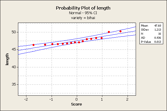
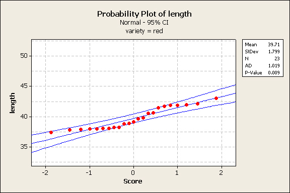
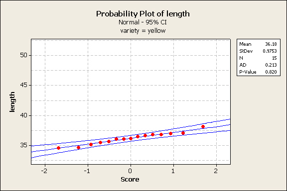
Exam #1 will be next Thursday, September 18. I've sent out an email asking each of you to let me know whether or not you will be available from 8:00-9:20 am on Thursday September 18 for this exam. Note that class normally starts at 8:30 am on Thursdays.
Here's a rough plan for next week:
One way to think about a density curve is that it represents a distribution for an idealized situation of infinitely many observations or values. The key property of a density curve is that the area under the graph between values a and b is equal to the proportion of observations/values in the distribution between the values a and b.
The most commonly used density curve distributions are the normal distributions. In class, we got some feel for the standard normal distribution by looking at problems on the Normal Distributions handout/worksheet.
I've assigned additional problems from Section 1.3. We'll start class tomorrow by addressing questions you bring on Section 1.3 problems. The new assignment includes the two problems on this handout.
Exam #1 will be next Thursday, September 18. I've sent out an email asking each of you to let me know whether or not you will be available from 8:00-9:20 am on Thursday September 18 for this exam. Note that class normally starts at 8:30 am on Thursdays.
I've have a few people come to my office to ask questions. I have time for lots more. Another source of help is tutors at the Center for Writing, Learning, and Teaching. Alison Paradise is the math faculty member who has hours at the CWLT this year. In addition, peer tutors are available for math (including statistics) and many other subjects. Details on the availability of peer tutors are on this page.We will have our first homework quiz at the beginning of class on Thursday. Here's a sample quiz to illustrate the style of questions you can expect. This quiz will focus on homework from Sections 1.1 and 1.2 as indicated in the "Quiz" column of the homework assignments above.
I have not assigned new homework problems for today so you should focus on making sure you understand ideas from Sections 1.1 and 1.2
We will have our first homework quiz at the beginning of class on Thursday. I'll give you a preview of this in class tomorrow.
I've assigned problems from Section 1.2. You'll need to read Section 1.2 to pick up a few ideas we have not yet talked about in class. In particular, one of the problems involves the "1.5×IQR rule for potential outliers". I am leaving it to you to read and apply this idea. We can address any questions you have on this in class on Monday.
We'll have a computer lab session for class one day next week so you can get some hands-on experience with Minitab. I'll let you know the schedule for this on Monday.
I've assigned additional problems from Section 1.1. In class, we talked about most of the ideas you'll see in this problems, but there are some details you'll need to read about in the text.
I've assigned a few problems from Section 1.1. We'll have more problems from this section after Thursday's class.
In class, we looked briefly at an online graphing tool that shows trends in baby names over time. It is available at The Baby Name Wizard.
Check out the Astronomy Picture of the Day.
You can look at exams from last time I taught Math 160. You can use these to get some idea of how I write exams. Don't assume I am going to write our exams by just making small changes to the old exams. You can use this old exam to prepare for our exam in whatever way you want. I will not provide solutions for the old exam problems.