| Section | Problems to do | Submit | Due date | Comments |
|---|---|---|---|---|
| 1.1 | 1.3,1.5-1.9,1.13,1.17,1.21,1.23,1.25 | 1.30 | Monday, January 25 | |
| 1.2 | 1.48-1.52,1.61,1.64 | None | None | |
| 1.2 | 1.47,1.53,1.65,1.73,1.78,1.79,1.91 | 1.80 | Thursday, January 28 | For Problem 1.73, you can do just the Cavendish density values. The rainwater pH data set is a bit too big for computing mean and standard deviation "by hand". |
| 1.3 | 1.99,1.100,1.107,1.109,1.111,1.112,1.114,1.115 | None | None | |
| 1.3 | 1.117,1.121,1.127,1.129,1.131,1.139 | 1.136 | Tuesday, February 2 | |
| 1.3 | 1.140,1.141,1.142,1.143,1.144,1.148 | None | None | Here are the normal quantile plots you'll need for Problem 1.148. |
| 3.2 | 3.49,3.53,3.55,3.57,3.60,3.67,3.70,3.71,3.76 | None | None | The Simple Random Sample applet is available on the textbook website. |
| 3.1 | 3.7,3,9,3.11,3.17,3.18,3.19,3.27,3.30 | None | None | |
| 3.3 | 3.83,3.84,3.85,3.86,3.91 | 3.95 | Tuesday, February 16 | |
| 3.4 | 3.103,3.105 | None | None | |
| 4.1 | 4.4,4.6 | None | None | |
| 4.2 | 4.16,4.18,4.21,4.22,4.25,4.29,4.31,4.33,4.36,4.37 | 4.34 | Monday, February 22 | |
| 4.3 | 4.47,4.48,4.52,4.59 | None | None | |
| 4.4 | 4.67,4,71,4.72 | None | None | |
| 4.4 | 4.79,4.81,4.83 | None | None | |
| 4.4 | 4.84,4.87,4.88,4.89,4.90 | None | None | There is a typo in Problem 4.89: The probability for age of death at 28 should be 0.00057 rather than 0.000057. |
| 5.1 | 5.11,5.13,5.15,5.19,5.21,5.27 | 5.28 | Tuesday, March 9 | |
| 5.1 | 5.22,5.25,5.29,5.33 | 5.24 | Thursday, March 11 | |
| 5.2 | 5.42,5.43,5.45,5.47,5.49,5.51,5.53 | None | None | |
| 6.1 | 6.13,6.17,6.23,6.25,6.29 | 6.26 | Friday, March 26 | |
| 6.2 | 6.36,6.37,6.55 | None | None | |
| 6.2 | 6.57,6.61,6.69,6.70,6.71 | 6.68 | Monday, March 29 | |
| 6.3 | 6.87,6.88,6.89,6.91,6.102 | None | None | |
| 7.1 | 7.1,7.2,7.3,7.4,7.15,7.25,7.32(a,b,c,d) | 7.36 | Tuesday, April 6 | |
| 7.1 | 7.21,7.33,7.39,7.41 | 7.34 | Thursday, April 8 | |
| 7.2 | 7.54,7.55,7.61,7.63,7.81 | 7.82 | Monday, April 12 | |
| 8.1 | 8.1,8.3,8.7,8.10,8.13,8.19,8.22,8.27 | 8.16 | Thursday, April 15 | |
| 8.1 | 8.30,8.31 | None | None | |
| 8.2 | 8.35,8.37,8.45,8.51,8.53 | None | None | |
| 9.3 | Handout problem | None | None | |
| 9.1 | 9.2,9.9,9.11 | None | None | |
| 2.5 | 2.107,2.108,2.109 | None | None | |
| 9.1 | 9.7 | 9.8 | Friday, April 30 | |
| 2.5 | Handout problems #4,5 | None | None | |
| 2.1 | 2.4,2.5,2.9,2.11,2.13,2.17,2.21 | 2.18 | Monday, May 3 | |
| 2.2 | 2.29,2.30,2.31,2.32,2.35,2.43 | None | None | You'll find the data file for 2.18 in the Jackson:Textbook Data:ch02 folder on the \\alexandria\stats network share. |
| 2.3 | 2.54,2.55,2.59,2.67,2.73,2.75 | None | None | Last set of problems! |
If you notice any broken links or if the daily note and assigned problems have not been updated in a timely fashion, send me a note so I can make corrections or updates as needed.
I will be available on a drop-in basis during office hours listed below. I'm also happy to schedule appointments for other times I am free. If you'd like to arrange an appointment, send me an e-mail or give me call (×3567).
Availability for Thursday, May 6:
Availability for Friday, May 7:
Availability for Monday, May 10:
Availability for Tuesday, May 11:
Exam #5 will be during our scheduled final exam period: 8:00-10:00 am on Wednesday, May 12. It will focus on material we have covered since the last exam. From the text, the relevant sections are 9.3, 9.1, 2.5, 2.1, 2.2, and 2.3 (in the order we covered them) with the exception of optional subsections. This handout has a list of specific objectives for the exam. For this exam, you can bring a calculator and one sheet (both sides) with notes and formulas.
I have pulled some problems from an old exam that are relevant to Exam #5. These problems deal with two quantitative variables (so material from Sections 2.1, 2.2, 2.3). Because of changes in the text from the previous edition to the current edition and differences in the length of fall and spring semesters, I do not have old exam problems that deal with two categorical variables (so material from Sections 9.1 and 2.5) or ``goodness of fit'' tests for one categorical variable (Section 9.3).
In class, we discussed our last topic, namely regression lines. A regression line is used when there is evidence of a linear association between two quantitative variables. The most common type of regression line is a least-squares regression line. The idea of least-squares regression is to find the line that minimizes the sum of squares of the difference between observed and predicted values for each data point. Some mathematics beyond the scope of our course can be used to find formulas for the slope and intercept of the least-squares line in terms of the means, standard deviations, and correlation for the X and Y distributions.
Here are two options for regression lines in Minitab:
Assignment #2 is due tomorrow.
Exam #5 will be during our scheduled final exam period: 8:00-10:00 am on Wednesday, May 12. It will focus on material we have covered since the last exam.
Today, we developed the idea of correlation for a linear association between two quantitative variables. We started by thinking about a "natural" coordinate system for a scatterplot that uses
For each point, we can compute "natural" (or "standardized") coordinate values. These tell us how many standard deviations the point is to the left or right of the horizontal mean and above or below the vertical mean. The correlation is an average of the product of these "natural" coordinates. This "natural" coordinate system breaks the scatterplot into four quadrants (I,II,III,and IV). Points in quadrants I and III "pull" the correlation in the positive direction whiles points in quadrants II and IV "pull" in the negative direction. So, a positive linear association has a positive correlation value while a negative linear association has a negative linear association.
To use Minitab to compute a correlation, go to Stat: Basic Statistics: Correlation...
Today, we looked at the idea of an association between two variables. In general terms, we say that two variables have an association if the distributions of one variable are not the same for all values of the other variables. Given data, we can use graphical views to look for a potential association.
Evidence for an association between two quantitative variables comes from the presence of a pattern (or patterns). One type of pattern is the presence of clusters. Sometimes the presence of clusters can be explained by a categorical variable. Another type of pattern occurs when the points tend to fall along a curve including the special case of a line. You should read Section 2.1 to pick up the relevant language to describe patterns in scatterplots, including form, direction, and strength.
Assignment #3 is due on Tuesday, May 4.
In class, we looked at an example that illustrates Simpson's paradox. This idea is discussed in Section 2.5 of the text. For homework, I've added two problems to the handout you worked on in class to help clarify how to resolve the apparent contradiction.
The optional Exam #4 redo is due at the beginning of class on Thursday.
In class, we looked at various proportions we can compute for a two-way table. Dividing individual counts by the table total gives the joint proportions. Dividing row totals or column totals by the table total gives marginal proportions. Dividing individual counts by row totals gives one kind of conditional proportions while dividing individual counts by columns totals gives another kind of conditional proportions.
These proportions are first introduced in Section 2.5 and then revisited in Section 9 so I have assigned problems from both parts of the text.
Exam #4 was returned in class today. For this exam, you have the option of redoing one problem as described on this handout. This is due at the beginning of class on Thursday, April 29.
In class, we worked through an example of inference for two categorical variables. The basic structure of a significance test is similar to what we did yesterday with a "goodness of fit" example. In particular, we have observed counts and then compute expected counts. With these in hand, we use the χ2 test statistic as a measure of the difference between the observed sample counts and the expected counts from the null hypothesis. The calculations can involve simple arithmetic but lots of it for a table of any size. Having computing technology available is very useful. In Minitab, we go to Stats: Tables: Cross-Tabulation and Chi-Square... or Stats: Tables: Chi-Square Test (Two Way Table in Worksheet)... depending on whether we have raw data or counts in hand.
Here are two possible interpretations of inference on a two-way table:
In our example, the first interpretation is more appropriate since the data we used came from samples drawn separately from the three populations defined by M&M type (plain, peanut, and peanut butter).
I've assigned problems relevant to Section 9.1. Note that the problems from Chapter 9 are not broken into sections. All of the problems are grouped together starting on page 548.
On Monday, we'll go back to some ideas from Section 2.5 (which we did not previously cover). In particular, we'll talk about joint, marginal, and conditional distributions for data in a two-way table. You'll encounter some of these phrases in reading Section 9.1.
We will finish the course by looking at the situation of having two variables measured on the individual things in one population. We will ask if there is an association between the two variables. We will start by looking at two categorical variables. For this, we will need a new tool, namely χ2 distributions (pronouced "chi-squared distributions").
In class, we introduced χ2 distributions in the context of doing inference for the distribution of proportions for a categorical variable. In this context, we still have only one variable to deal with. The variable is categorical with two or more values (or categories). We've previously dealt with the case of two categories ("success" and "failure") so the interesting thing is to work with three or more categories. We use color for plain M&M's as our example in class. The type of significance test we did in class is often called a "goodness of fit" test. This material is covered in Section 9.3 of the text. We are starting with this in order to get experience with χ2 distributions without adding other new ideas.
Assignment #3 is due on Tuesday, May 4.Exam #4 will be tomorrow. It will cover material from Chapters 7 and 8 with the exception of optional sections and subsections. This handout has a list of specific objectives for the exam. For this exam, you can bring a calculator and one sheet (both sides) with notes and formulas.
Today, we met in the computer lab for hands-on practice with Minitab. As part of this, you had Minitab carry out the calculations for Problem 8.37. We then distributed Assignment #3 and you got started on setting up and exploring the relevant data set. Assignment #3 is due on Tuesday, May 4.
Exam #4 will be on Tuesday, April 20. It will cover material from Chapters 7 and 8 with the exception of optional sections and subsections. This handout has a list of specific objectives for the exam. For this exam, you can bring a calculator and one sheet (both sides) with notes and formulas.
Today, we looked at inference for comparing proportions for two populations. In particular, you worked out an example of computing a confidence interval for the difference in two population proportions. In some situations, we might carry out a significance test on the null hypothesis that the two population proportions are the same versus either the two-sided alternative or a one-sided alternative. You'll need to read about this in Seciton 8.2 of the text. Pay attention to the use of the pooled estimate used in computing the standard error under the null hypothesis. The main idea here is to use the assumption that both populations have the same proportion so the two samples can be thought of as coming from the same population and thus pooled into one large sample for the purpose of estimating the unknown population proportion.
For class tomorrow (Friday, April 16), we will meet in the computer lab Mc324. You can go directly there rather than to the usual classroom.
Exam #4 will be on Tuesday, April 20. It will cover material from Chapters 7 and 8 with the exception of optional sections and subsections.
In class, we looked at using Minitab to do the calculations for inference on a proportion. We also discussed how to determine a sample size in advance to get a specified margin of error. I've assigned two additional problems from Section 8.1 on this idea.
Exam #4 will be on Tuesday, April 20.
Today, we looked at inference for the proportion of a value for a categorical variable. The basic structures of confidence intervals and significance tests are the same as we've seen in past contexts. The details come from what we have previously seen about sampling distributions for proportions.
In Section 8.1, there is a "Beyond the Basics" subsection starting on page 491 and ending on page 493 that we will not cover.
Exam #4 will be on Tuesday, April 20.
In class, we focused on solidifying understand of inference for comparing means of a quantitative variable for two populations, principally by working through Problem 7.81 carefully.
On Monday, we will turn our attention to categorical variables and inference for proportions. Most of the broad patterns we saw this week should be recognizable in what we do next week.
For today, I need to reschedule office hour to 3:00-4:00 (from the usual Thurday time of 1:00-2:00).
Today, we looked at inference for comparing means of a variable for two populations (so: one variable, two populations). In this context, the basic structure of inference should be familiar. In the details, there are several small new ideas including (a) combining standard errors for separate sample means to get the standard error for the difference in sample means and (a) determining an appropriate value for degrees of freedom in the relevant t-distribution. In terms of (b), you can use approximation #2 given on p. 451 when doing calculations by hand. Minitab will use approximation #1. (If you are curious about the details, the underlying formula is given on page 460. You are not responsible for knowing or using this formula.)
In class, we discussed significance tests within this new context. We did not explicitly discuss confidence intervals for this context so you will need to read about these in the text. There should be no surprises in how to construct a confidence interval here. The basic plan is familiar and the new details are the same as the ones we used in our discussion of significance tests.
In reading Section 7.2, note that it ends with some optional subsections (marked by asterisks) that we will not cover.
In class, we discussed the idea that our initial justitication for the validity of t procedures was based on an assumption that the population distribution is normal. Without access to the full population, we need to make a judgment about normality based on evidence from the sample distribution (and experience with similar types of data if we have that level of experience). In practice, t procedures can work well even with a non-normal population distribution. Guidelines for appropriate use of t procedures are given in the text (and on the slide we viewed in class).
We also looked at how to use Minitab to compute confidence intervals or P-values. Go to Stat: Basic Statistics: 1-Sample t.... In the dialog box that comes up, you have a choice between Samples in columns or Summarized data. Use Samples in columns if you have data in a worksheet. Use Summarized data if you already know the sample mean and sample deviation. You also have a check-box option for Perform hypothesis test. If you turn on this option, you will need supply a value for the Hypothesized mean. You can go to Options... to change the confidence level (default is 95%) or select the type of alternative hypothesis (default is two-sided).
For Thursday, I need to reschedule office hour to 3:00-4:00 (from the usual Thurday time of 1:00-2:00).
After looking at questions from Section 7.1 problems, we used the context of Problem 7.32 as an example of doing a significance test where the test statistic is t-distributed. The basic structure of a signficance test is the same as our previous experience. The only difference is that we are now working with a new distribution for the underlying sampling distribution. Using standard error as an estimate of standard deviation for the sampling distribution leads to using a t-distribution (with the appropriate degrees of freedom) in place of the standard normal distribution.
I've assigned some more problems from Section 7.1 that deal with significance tests for means.
Here are tentative dates for the remaining exams we have:
Note that the last of these is on the Wednesday of final exam week.
Prior to the exam, we were looking at the general idea of inference using a somewhat artificial setting in order to avoid introducing a new set of ideas needed for more realistic settings. Now that we have some experience with confidence intervals and significance tests in that simple but artificial setting, we can turn our attention to more realistic settings.
In class, we started in on this by looking at inference for a population mean μ when we do not know the population standard deviation σ. Once we have a sample in hand, we can compute the sample standard deviation s and then use this as an estimate of the unknown population standard deviation σ. So, we replace the sampling distribution standard deviation σ/√n with the standard error s/√n. The distribution of statistics based on using the standard error differs from the distribution of statistics based on using the standard deviation. So, we needed to learn about some new distributions, namely t-distributions. To get a confidence interval in this context, we need to know the multiplier t* from the relevant t-distribution. Table D gives us these multipliers for various t-distributions and various confidence levels. (Note that Table D is organized by "upper-tail probabilities" so we need to relate a given confidence level to the corresponding upper-tail probability. A confidence level of 95% corresponds to an upper-tail probability of 2.5% or 0.025.)
I've assigned some problems from Section 7.1. These deal with confidence intervals in the new context. On Monday, we'll look at significance tests in this new context.
Exam #3 will be on Thursday, April 1. It will cover material from Chapters 5 and 6 with the exception of optional sections/subsections (including all of Section 6.4) and the "Beyond the basics" sections. This handout has a list of specific objectives for the exam
For the exam, you can bring a calculator and a note card with formulas. You can also bring your own paper if you prefer that over the blank copy paper I'll provide.
In class, we looked at a draft handout showing the relationship between population distribution, a sample distribution, and the sampling distribution for means. I've polished that up a bit and there is a link to it above. There is also a link to a analogous handout for proportions.
On Wednesday, I have some times available in the morning and in the afternoon. Contact me if you'd like to set up a time to come ask questions.
In the process of looking at problems from Section 6.3, we looked at some issues that arise in carrying out and interpreting significance tests. As part of this, we used Problem 6.95 to provide an example of distinguishing between statistical significance and practical importance.
Exam #3 will be on Thursday, April 1. It will cover material from Chapters 5 and 6 with the exception of optional sections/subsections (including all of Section 6.4) and the "Beyond the basics" sections. This handout has a list of specific objectives for the exam
We spent our time in class going carefully through several homework problems that involving carrying out significance tests. You should aim to very soon be comfortable with the mechanics of carrying out significance tests so that you can focus on the meaning of significance tests. Section 6.3 provides some advice on how to properly interpret significance tests. I've assigned a few problems from this section. You'll benefit from reading through Section 6.3 before looking at the assigned problems.
Assignment #2 is due on Monday, March 29.
Exam #3 will be on Thursday, April 1.
In class, you worked through the same significance test example we did together in class on Tuesday using your own sample from this handout. You can check your results on this version of the handout that includes the z-score and P-value for each sample.
I've assigned another set of problems from Section 6.2.
Assignment #2 is due on Monday, March 29.
Exam #3 will be on Thursday, April 1.
Today, we had our first look at significance tests. The reasoning of significance tests can be uncomfortable at first; it becomes easier with experience. Here's the outline we stepped through in class with an example:
I've assigned a few problems from Section 6.2 that deal with setting up null and alternative hypotheses. The example we worked through in class used the two-sided alternative hypothesis. In some situations, a one-sided alternative hypothesis is used. You'll need to read about this in text.
I've also posted the Section 6.1 problems that I neglected to put up yesterday. You should work on the Section 6.1 and Section 6.2 problems before Thursday's class.
Assignment #2 is due on Monday, March 29.
Exam #3 will be on Thursday, April 1.
At the beginning of class, I (finally) returned Assignment #1. Here's the handout with notes on common issues. For reference, here's two examples of well-done reports:
In class, we reviewed the reasoning behind confidence intervals and then each of you worked out an example of a 95% confidence interval from this worksheet. In the context of the worksheet, we could determine the true value of the parameter (a population mean in this case). With about 20 different 95% confidence intervals, it should not be surprising that one or two would fail to contain the parameter value. For the 18 confidence intervals from the class as a whole, it did turn out that 17 contained the parameter value while one did not. This is the nature of confidence intervals: they are produced by a random process that has a fixed probability of generating an interval containing the true parameter value. In practice, you would only have sample in hand and thus only one confidence interval. There is no way to know whether or not the confidence interval you get contains the true parameter value.
I have assigned problems from Section 6.1 that you should work on before class tomorrow.
Assignment #2 is due on Monday, March 29.
In class, we looked at an overview of statistical inference. The general idea of inference is to use information on a statistic value from one sample to infer something about the value of the corresponding parameter for the population from which the sample was drawn. Because selecting a sample and computing a statistic value is a random process, we must account for variability in the distribution of all possible statistic values. So, inference consists of reporting a statistic value as an estimate of the unknown parameter value and reporting something else that has information about the variability. We will study two main methods of inference: confidence intervals and significance tests. In a confidence interval, sampling variability is accounted for with a margin of error. In a significance test, sampling variability is accounted for with a P-value.
All of this may feel somewhat abstract until we get deeper into the specifics. In many ways, a main goal for the remainder of this course is to be able to read the preceeding paragraph with meaning.
I have not assigned additional problems from Section 6.1. I'll do this after class on the Monday following break.
Enjoy your break!
We used most of today's class session to discuss problems from Sections 5.1 and 5.2. Tomorrow, we will begin looking in detail at statistical inference. Understanding inference is one of the primary goals for this course.
At the end of class, we returned to the sampling distribution simulation applet to generate more two more conjectures:
The second of these conjectures is made precise in the Central Limit Theorem.
I have added Problem 5.49 to the assigned problems from Section 5.2
Assignment #2 is due on Monday, March 29.
Here are tentative dates for the remaining exams we have:
Note that the last of these is on the Wednesday of final exam week.
In class, we looked at sampling distributions for means. For some time, we've been doing this through simulations using this applet. From these simulations, we have been able to conjecture two things:
Using our knowledge of random variables, we were able to confirm these conjectures and provide a formula to directly relate the standard deviation of a sampling distribution for means to the standard deviation for the population and the size of the samples.
After looking at questions from Section 5.1 problems on sampling distributions for counts, we turned our attention to sampling distributions for proportions. Sampling distributions for proportions are closely related to sampling distributions for counts since a proportion is just a count divided by the sample size. The sampling distribution for proportions is just a binomial distribution B(n,p) with the horizontal axis scaled by 1/n and the vertical axis scaled by n. (Scaling the vertical axis by n keeps the total area equal to 1.)
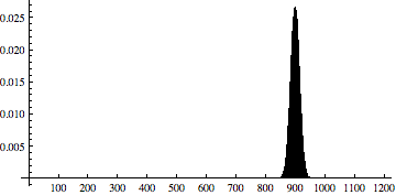
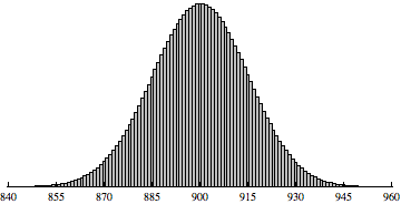
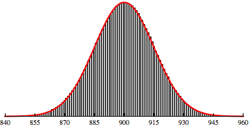
In class, we also talked briefly about the context for Problem 5.28 that is due tomorrow. In that problem, the relevant distribution is B(1200, 0.75). Here's two views of the probability histogram for this binomial distribution:
The view on the left shows the full range of values from 0 to 1200. For most of this range, the probabilities are essentially zero. The view on the right zooms in on the interesting part of the distribution. In the zoomed-in view, we can see that this binomial distribution is well approximated by a normal distribution, specifically N(900,15). To make this even more obvious, here's a view showing both B(1200,0.75) (the histogram bars) and N(900,15) (the red curve):
In class, we continued discussing binomial distributions B(n,p) as models for the count of successes in n observations with success probability p on each observation. The binomial model is exact if the observations are independent. If we draw a SRS of size n from a population (without replacement), then the observations are not independent so the binomial model is not exact. However, the binomial model is a good approximation if the population is large compared to the sample size. In particular, we will use the binomial model if the population is at least 20 times bigger than the sample.
Today, we looked at three aspects of binomial distributions:
On Monday, we'll look at sampling distributions for proportions. Since the proportion of successes is just the count of successes divided by the sample size, we'll be able to use what we now know about sampling distributions for counts.
Today, we began looking at sampling distributions for counts. We started with data collected by hand and by computer simulation for the sampling distribution for counts in n=5 observations in which each observation has a success probability of p=0.2. In our data collection by hand, "success" meant getting a pink square. Using our knowledge of probability, we were also able to derive a model for this sampling distribution. The model we got is an example of a binomial distribution. We saw good agreement between the data (for a large number of samples) and this binomial distribution. At the end of class, we talked briefly about generalizing this model to different values of n and p. We'll continue this tomorrow.
I have not yet assigned problems from Section 5.1. I'll do this after tomorrow's class in which we talk more about binomial distributions. For now, you should read through Section 5.1 to get a general sense of the topics we'll be discussing.
Our goal today was to prepare for tomorrow's exam. The exam will cover material from Chapters 3 and 4 (except Section 4.5). For the exam, you can bring a calculator and a 3" by 5" index card with formulas. The handout we looked at in class gives one way of organizing the material for this exam. This list of specific objectives for the exam gives more details.
Things you can do to prepare well for an exam include
You should seek to go beyond mastering mechanical aspects (such as computational skills) to mastering concepts and ideas. For example, in doing homework problems, ask yourself ``Do I understand the ideas and skills required to get a correct answer?'' rather than merely ``Did I get the correct answer?''
Problem 4.89 illustrates how the law of large numbers is relevant to thinking about the business of insurance. In class, we looked at simulations of the situation for this problem. For reference, this handout has plots similar to the ones we generated in class.
In class, we also talked about one last idea, namely how the mean and standard deviation of a random variable change under a linear transformation. A linear transformation Y=bX+a is just a scaling of each value through multiplication by the factor b followed by a shifted through addition of the amount a. Both the scaling and the shifting also change the mean in the same way so we have μY=bμX+a. The scaling affects the standard deviation and variance but the shifting does not so we have σY=bσX and σY2=b2σX2.
The linear transformation rules for mean, variance, and standard deviation come into play if we change units. A more important use of the rules comes when we look at how the mean and standard deviation of sample means for SRSs of size n are related to the population mean and the population standard deviation. We finished class with an example of this. We'll follow up on this after the exam.
I've added one problem (4.84) to the last set of problems from Section 4.4.
Exam #2 will be on Tuesday, March 2. It will focus on material we've covered since the previous exam. The relevant text material is from Chapters 3 and 4 (with the exception of Section 4.5). This handout has a list of specific objectives for the exam.
In class, you played a very simple gambling game to set up a discussion of running mean and the law of large numbers. In each play of the game, your net gain was -$1 (with probability 1/2), $0 (with probability 1/3), or $2 (with probability 1/6). We defined the running mean as the mean of all the times you've played up to a certain round. For example, the running mean after two rounds is the mean net gain for those first two rounds which you compute by adding the net gains for the two rounds and then dividing by two. The running mean after 10 rounds is the mean net gain for those ten rounds which you compute by adding the net gains for the 10 rounds and then dividing by 10. So, the running mean is a function of how many rounds you've played. Since net gain is a random variable, we can also compute the random variable mean.The random variable mean can be thought of as the mean for the idealized sitaution of infinitely many rounds. It is reasonable to think that the running mean for finitely many rounds will become closer to the idealized random variable mean as the (finite) number of rounds increases. This intuition is correct and is formalized in the law of large numbers. The law of large numbers is a mathematical theorem that guarantees the running mean will get, and stay, close to the random variable mean as the number of rounds gets large.
The law of large numbers can be useful in thinking about gambling games, insurance, and investments. I've assigned some problems from Section 4.4 that are set in the context of insurance.
Exam #2 will be on Tuesday, March 2.
In class, we first talked about the distinction between discrete random variables and continuous random variables. For a discrete random variable, we can list the values and corresponding probabilities. For a continuous random variable, we can assign probabilities to intervals of values and represent those probabilities as areas under a probability density curve. There is a close connection between probability density curves we are now exploring and the density curves for model distributions we saw earlier in the course. Recall that a model distribution describes the values of a variable thought of as measured on an ideal population that is infinitely large. The connection comes from the fact that the following two things are equal:
This is much easier to understand within the context of a specific example. If we assume that birth weights (for current full-term U.S. babies) are normally distributed with a mean of 7.6 pounds and a standard deviation of 2.1 pounds, then the following two things are equal:
We also started a second topic today, namely how to compute the mean, variance, and standard deviation of a random variable Z that is the sum of two other random variables X and Y when we know the means, variances, and standard deviations of X and Y.
Exam #2 will be on Tuesday, March 2.
In class, we looked at two examples of computing mean and standard deviation for a discrete random variable. Later this week, we'll talk about how mean and standard deviation are computed for a continuous random variable.
Questions on Section 4.2 problems and the "shared birthday" problem have given us practice with the basic rules of probability. If you do not yet feel comfortable using the rules accurately and efficiently, you should work on more problems and examples to quickly master these basics.
In the last part of class, we begin discussing random variables. In particular, we explored an example to illustrate how to compute the mean and standard deviation of a discrete random variable. We'll get more practice with this on Monday.
I've assigned a few problems from Section 4.3. For some of these, you'll need to understand some ideas from Section 4.3 that we only briefly mentioned in class today.
In class, we discussed the basis rules of probability. You should aim to quickly become accurate and efficient with these rules. Working on the problems from Section 4.2 will give you some practice.
In class, you collected data on some random processes (rolling dice, flipping coins). We'll refer to this data as we continue exploring randomness and probability.
I've assigned a few problems from Section 4.2. On Thursday, we'll talk about more of the details from Section 4.2 and then I'll assign additional problems (including one or two to submit).
Assignment #1 is due in class on Thursday.
I have assigned a few problems from Section 3.4 that consider some ethical issues connected to experimental and observational studies.
In class, we introduced the basic idea of a random process and associated probabilities. I've assigned a few problems from Section 4.1. Tomorrow, we'll start a more in-depth study of probability.
Assignment #1 is due in class on Thursday.
Today, we had a computer lab session to get some familiarity with Minitab. If you were unable to come to class today, you should work through the lab session handout on your own. You can find Minitab on computers in various labs and dorm lounges around campus. Come ask if you have questions or get stuck.
I also distributed a handout for Assignment #1. This assignment is due in class on Thursday, February 18.
In class, we set up the general framework for statistical inference by looking at two examples. You should work to quickly become comfortable and precise in using the terminology of population, parameter, sample, and statistic.
We also looked at this sampling distribution applet. The story told in the applet illustrates one of the central themes for our course.
Here are tentative dates for the remaining exams we have:
Note that the last of these is on the Wednesday of final exam week.
Remember that we will meet in the computer lab (MC 324) for class tomorrow. You can go straight there rather than to the usual classroom.
In class, we looked at some fundamental ideas in experimental
studies within the context of a particular example. For reference in
case you are interested in learning more about that example, the journal
article we looked at is available online through the UPS Library:
"A controlled trial of arthroscopic surgery for osteoarthritis of the knee"
J Bruce Moseley, Kimberly O'Malley, Nancy J Petersen, Terri J Menke, et al.
The New England Journal of Medicine. Boston: Jul 11, 2002. Vol. 347, Iss.
2; pg. 81.
To access this link, you will need to be using a computer on the UPS campus
network. If you are off-campus, you might be able to access the link after
entering your UPS login name and password in a dialog box (for something
called a "proxy server").
We will be skipping over the material in Chapter 2 for now. We'll come back to it at the end of the semester. For now, we will start exploring the ideas in Chapter 3 on collecting data in a way that allows for statistical inference. Learning the basics of statistical inference is the main goal of this course.
Much of the material in Chapter 3 is descriptive. We will not discuss all of the details in class so you will be responsible for reading the text carefully and asking questions to clarify details as needed. Before class tomorrow, you should read the Introduction to Chapter 3 and Section 3.2. I've also assigned a few problems from Section 3.2 that you should work on before class tomorrow.
In class today, we discussed some basic issues related to sample surveys. A fundamental idea here is that of a simple random sample. There are variations on simple random samples that you should read about in Section 3.2.
Exam #1 will be tomorrow (Friday, February 5). It will cover material from Chapter 1 in the text. This handout has a list of specific objectives for the exam.
As a guide to expectations on exam questions, here are some student responses to certain problems from the Fall 2008 Math 160 Exam #1.
Exam #1 will be on Friday, February 5. It will cover material from Chapter 1 in the text. This handout has a list of specific objectives for the exam.
I design exams so that approximately three-fourths of the point value is for problems that are ``straightforward'' and the remainder involves more challenging problems. By this, I intend that a well-prepared student can do the ``straightforward'' problems without hesitation. These problems may be similar to assigned homework problems. The more challenging problems may involve applying, generalizing, or synthesizing relevant ideas.
Things you can do to prepare well for an exam include
You should seek to go beyond mastering mechanical aspects (such as computational skills) to mastering concepts and ideas. For example, in doing homework problems, ask yourself ``Do I understand the ideas and skills required to get a correct answer?'' rather than merely ``Did I get the correct answer?''
In class, we looked at getting percentiles for normal distributions and then used this idea in constructing normal quantile plots. Normal quantile plots are a tool for judging whether or not it is reasonable to think of a data distribution as having come from normal distribution. For now, you can focus on interpreting normal quantile plots rather than on constructing them. For reference, here are instructions on using Minitab to build normal quantiles plots.
Exam #1 will be on Friday, February 5. It will cover material from Chapter 1 in the text.
Our focus in class today was learning how to get areas/proportions for normal distributions. Options include
If we need areas/proportions for a non-standard normal distribution, we can compute a z-score and then look for the area for that value in the standard normal distribution table.
To get normal distribution areas/proportions on a TI-83 or TI-84, go to the DISTR menu and select normalcdf(. You'll need to enter values with the syntax
normalcdf(lower value, upper value, mean, standard deviation)
If you want the area to the left of a given value, you can use something like -1000 for the lower value.
To get proportions for normal distributions in Minitab, go to Calc: Probability Distributions: Normal.... Make sure the option Cumulative probability is selected. You'll need to enter a mean and a standard deviation. You can then select the option Input constant: and fill in the relevant value.
Exam #1 will be on Friday, February 5.
After reviewing the general ideas of density curve and model distribution, we focused on normal distributions. These are the most important distributions we will use in this course. You should work to quickly become comfortable with normal distributions. I've assigned problems from Section 1.3. For the ones that involve a normal distribution, you should need only the 68-95-99.7 rule. Tomorrow, we'll talk about how to find more general areas/proportions for normal distributions. I'll then assign additional problems from Section 1.3 including at least one to be submitted.
Exam #1 will be on Friday, February 5.
In the last part of class, we began looking at density curves. You can think about a density curve as representing an idealized distribution with infinitely many values. The area under a density curve for a particular interval gives the proportion of values that fall into that interval. On Thursday, we'll continue talking about density curves with particular focus on density curves for normal distributions. For now, I've assigned just two problems from Section 1.3.
Exam #1 will be either Thursday, February 4 or Friday, February 5. I'll set a specific date before our next class.
In class, we looked at mean and standard deviation as measures of center and spread, respectively. I've assigned additional problems from Section 1.2. I've separated these out above so you can more easily see what's new.
You should take the time to compute mean and standard deviation "by hand" for a few examples. (Here, "by hand" can involve using a calculator for the arithmetic but not using a built-in mean or standard deviation function.) Once you understand how to calculate these numbers, you can turn to technology to speed up the process. We'll talk in class tomorrow about expectations for exams in term of calculating "by hand".
For a unimodal distribution, we want measures of center and spread. Two common choices are
We looked at median and IQR in class today. We'll discuss mean and standard deviation in class on Monday.
I've assigned some problems from Section 1.2. You'll need to read Section 1.2 to pick up a few ideas we have not yet talked about in class. In particular, one of the problems involves the "1.5×IQR rule for potential outliers". I am leaving it to you to read and apply this idea. We can address any questions you have on this in class on Monday.
I'll assign more problems from Section 1.2 (dealing with mean and standard deviation) after Monday's class.The Center for Writing, Learning, and Teaching (CWLT) has tutoring help available for many subjects. For statistics, help is available from peer tutor Thor Ruskoski and from faculty member Chuck Hommel. Thor's hours are 11am-1pm Monday and 2-4pm Wednesday by appointment and noon-1 pm Friday on a drop-in basis. I'll post Chuck Hommel's hours soon. To make an appointment, you can stop by the CWLT or call 253-879-2960.
We are distinguishing between two types of variable: categorical and quantitative. Describing a distribution of a categorical variable is straightforward. We need only count the number of values for each category (for example, 12 female, 11 male). Counts can be displayed in a bar chart. From these counts, we can compute proportions or ration. Proportions are sometimes displayed in a pie chart.
For a distribution of a quantitative variable, we generally need to work a bit harder, particularly if the distribution has many values (hundreds, thousands, ...). For a small distribution, a stemplot is a quick and easy way to get a visual sense. More often, we will use a histogram for a visual description of a distribution.
With a picture (stemplot or histogram) in hand, we can ask about the shape of the distribution:
Answering these questions can involve judgment. With a histogram, that judgment might depend on how the binning is set up.
I've assigned problems from Section 1.1, including one to submit on Monday. We'll start class tomorrow by addressing questions you have on the assigned problems. Typically, we will not discuss problems to be submitted in class but you can come discuss those problems with me outside of class.
In class, we began developing some basic terminology for dealing with data. In particular, we used the terms variable, type, range, and values. The range of a variable is the set of all possible values. For a categorical variable, it is often straightforward to list the range. For a quantitative variable, determing a precise range can be hard but there are generally some obvious restrictions on the range that can be stated. In class, for example, we looked at the variable hand span (in cm). This is a quantitative variable with a range that is restricted to positive numbers. (A more subtle point is that range might be determined by the thing we are measuring and the way in which we measure. For example, actual hand span values could be any positive number. If we are measuring with a ruler and rounding to the nearest 0.1, these measured hand span values would be positive numbers in steps of 0.1 rather than all positive numbers.)
I've assigned two problems from Section 1.1. After Thursday's class, I'll assign more problems from this section, including one or two to submit.
You can look at exams from last time I taught Math 160. You can use these to get some idea of how I write exams. You can use these old exams to prepare for our exams in whatever way you want. I will not provide solutions for the old exam problems.
Don't assume I am going to write our exams by just making small changes to the old exams. Also note that we were using a different edition of the textbook at the time so there may be small differences in the ordering of topics, language, and notation.