

| Section | Problems to do | Target date | Comments |
|---|---|---|---|
| 1.1 | 1,2,3,4,5,6,7,9 | Tuesday, Sept 1 | |
| Gaussians | 1,2 | Friday, Sept 4 | |
| Flux | 1,2,3 | Thursday, Sept 10 | |
| 1.2 | 1,4,5,6,7,8,10 | Monday, Sept 14 | For #8, you can now move on to solving the PDE model. |
| 1.3 | 1,4,5,6,7 | Friday, Sept 18 | |
| 1.5 | 3,4,5 | Monday, Sept 21 | |
| 1.9 | 1,2,3,5 | Thursday, Sept 24 | |
| 2.1 | 1,2,3,4,5 | Monday, Oct 5 | See note for October 2. |
| 2.4 | 1,2,3,4 | Monday, Oct 12 | |
| 2.2 | 2,3,4 | Monday, Oct 12 | For Problem 2, evaluate the integral in (2.14) for the given initial velocity. |
| 3.2 | 1,2,3,4,5,6,8 | Thursday, October 22 | Problem 7 (not assigned) concerns wavelets. This would be a good project topic. |
| 3.3 | 1,2,3,5 | Friday, October 29 | |
| 3.4 | 3,6,7,9 | Monday, November 9 | |
| 4.1 | 1,2,3 | Tuesday, November 10 | |
| 4.2 | 1,2,4 | Monday, November 15 | |
| 4.3 | 1,2 | Tuesday, November 24 | |
| 4.4 | 1,3 | Tuesday, December 1 |
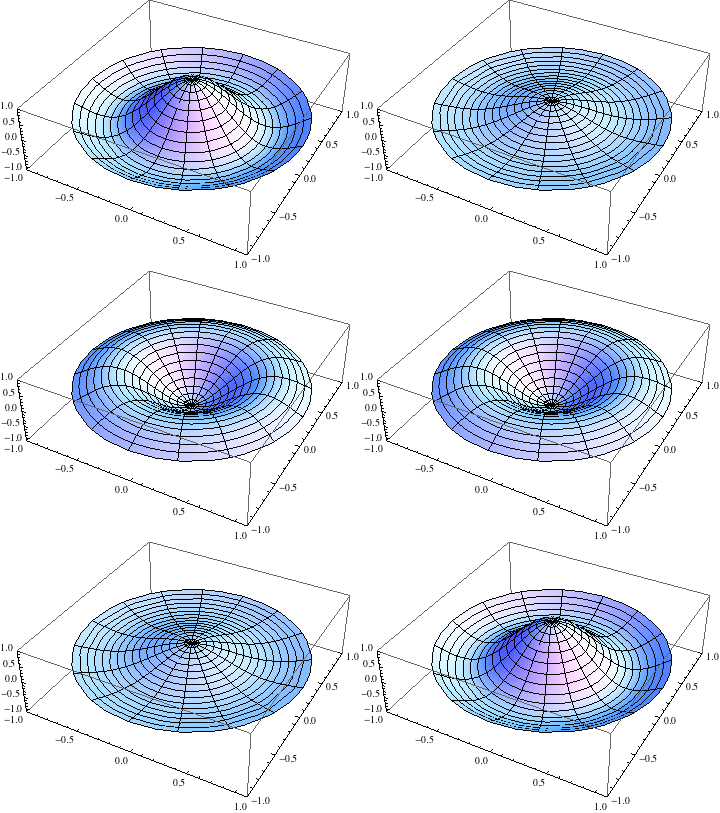
The Mathematica notebook posted for today has a section with the more efficient coding of animations for circularly symmetry normal modes of a circular drumhead. A second section uses the same ideas for more general normal modes.
Have a good Thanksgiving break!
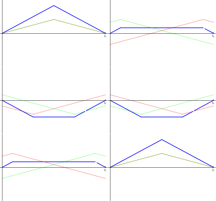
After class, Nathan suggested a way to make Mathematica more efficiently compute the animations we were trying in class. I'll annotate the Mathematica notebook and post it soon. In the meantime, here's an animation of the n=2 normal mode for circularly symmetric vibrations on a circular drumhead:

Section 4.5 of the text looks at the heat equation on a disk in the circularly symmetric case. In class, we are looking at the wave equation on the disk in circularly symmetric case. Both problems lead to Bessel functions of order zero so you can read Section 4.5 to complement what we are doing in class.
In class, we started in on a BVP for Laplace's equation on a disk. As part of this, we needed to express the Laplacian uxx+uyy in polar coordinates. Using the chain rule, we arrived at the polar coordinate form of the Laplacian as urr+(1/r)ur+(1/r2)uθθ. We then started in on our "product solution→separation of variables→SL problem→orthogonal expansion" approach. We'll finish this off tomorrow.
I've assigned problems from Section 4.2. We can address questions on Section 4.1 and 4.2 problems in class on Monday.
Exam #9 is due on Friday November 20. Note that you have a choice of two problems.
I've posted problems from Section 4.1.
If you have not already talked with me about a project topic, do so soon. Here's some additional possibilities:
In class, you analyzed the Sturm-Liouville problem on this handout. The eigenvalues turn out to be determined by an equation that cannot be solved exactly so we must resort to numerical approximation. Details are in today's Mathematica notebook.
Problems from Section 3.4 have been posted.
Many properties of eigenvalues and eigenfunctions for a regular Sturm-Liouville problem parallel properties of eigenvalues and eigenvectors for a real symmetric matrix.
In class, we started solving an IBVP for the heat equation. The basic plan is to look for solutions in the form of products. We then make a separation of variables argument to get two ODE problems. One of these is a second-order ODE together with two boundary conditions. This is an example of a Sturm-Liouville problem. Tomorrow, we'll look at the general Sturm-Liouville problem.
In class, I misspoke in referring to the "power spectrum" when I should have said frequency spectrum.
In class, we are using a convention for the zeroth Fourier coefficient that differs from what the text uses. The text includes the function 1 in with the cos(nx) functions as the n=0 case. The coefficient a0 as computed using the formula for an differs from a factor of 2 from a0 as computed separately. This factor of 2 is the difference between the normalization factor of 2π for 1 and the normalization factor of π for cos(nx) (n=1,2,3,...). Since the text computes a0 using the normalization factor of π, the factor of 2 must be put in elsewhere. This explains the presence of the 2 in the denominator of the first term of Equation (3.17) on p. 107 of the text.
In class, we looked at the idea of complete orthogonal sets. An orthogonal set is complete in a vector space if no other nonzero vector is orthogonal to each vector in the set. In many vector spaces, incuding L2(a,b), a complete orthogonal set serves as a basis.
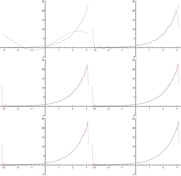
As our first example of a complete orthogonal set, we look at {sin(nx)}∪{1}∪{cos(nx)} in L2(-π,π). The expansion of a function in terms of this complete orthogonal set is known as the (classical) Fourier series expansion. We look at the example of expanding the exponential function in a classical Fourier series expansion. The following animation shows partial sums for this expansion starting with n=1 and ending with n=50. (For each step, a pair of cos(n x) and sin(nx) terms are added).

I've assigned one problem from Section 3.3. I'll assign more after Thursday's class.
We started class with a look at Section 3.2 Problem 3. This problem involves using the Gram-Schmidt process to generate an orthogonal set in L2(-1,1) starting with the set {1,x,x2,...}. The Mathematica notebook for today has the related calculations.
We finished with a somewhat detailed calculation from which we can conclude the following: the Fourier coefficients minimize the mean-square difference between a function and any partial sum for the expansion of that function in terms of an orthogonal set.
So far, we have looked only at the orthogonal set {sin(nx)} in L2(-π,π). The set {sin(nx)} is not a basis for L2(-π,π) since there are function is L2(-π,π) that cannot be expanded in terms of {sin(nx)}. (As an example, try expanding an even function such as f(x)=1.) Next week, we'll look at a bigger orthogonal set in L2(-π,π) that includes sines and cosines. This bigger set is a basis for L2(-π,π) meaning we can expand any function in L2(-π,π) as an infinite series of the basis functions.
We are currently looking at orthogonal expansions. The general context is a vector space for which we have a given inner product. We find (or build) a basis for the vector space that is orthogonal with respect to the inner product. To expand some other vector (from the vector space) in terms of the orthogonal basis, we can compute the coefficients (as opposed to solving a system of equations to get the coefficients). In particular, we will need to work with orthogonal expansions in the vector space L2(a,b). Here are a few notes on L2(a,b).
There are a lot of ideas in Section 3.2. I've assigned problems from this section. You should attempt at least the first few of these before our Thursday October 22 class.
You should begin thinking about a topic for your course projects. This handout has details on expectations and requirements for the project. You will need to have a topic approved by Friday, November 20.
In the computer lab yesterday, we looked at an example of expanding a given function in a linear combination of sine functions. Today in class, we backed up to a simpler context, namely expanding a given vector in ℜ3 in a linear combination of basis vectors. To compute the expansion coefficients, we generally need to solve a system of three equations in three unknowns. However, if the basis is orthogonal, we can easily compute the coefficients rather than solve a system of equations. Tomorrow, we'll generalize from the context of vectors in ℜ3 to vectors in a particular function space. (That is, the abstract vectors will be functions having certain properties.)
The link above connects to the Mathematica notebook we looked at in class. I have been experimenting with how to make dynamic content (such as Manipulate and Animate objects) available in Mathematica Player. If you have been using Mathematica Player, try downloading this test file. Let me know whether or not the dynamic content works in Mathematica Player. (Note: This test file just has one piece from today's notebook.)
We are going to skip over the rest of Chapter 2 for now. If time permits, we'll circle back toward the end of the semester to talk about integral transform approaches to solving PDEs on unbounded domains.
Our focus will now turn to PDEs on bounded domains. We started by thinking about the heat equation on a bounded interval (in the spatial variable). We looked at a reasonable first approach, namely trying to define a related Cauchy problem by extending the initial condition from the bounded interval to the entire line in some way that the boundary conditions will be satisfied. This seems not to be feasible. An approach that does work requires us to develop a new mathematical idea. We introduced this idea by playing around with a specific example. We'll use ideas from this example in developing a general approach to the problem of approximating a given function with a sum of other sines (and sums of other sets of functions).
In class, we worked out the solution for Problem 3 of Section 2.2. When we worked out the details for a specific "signal" function (namely s(t)=sin(t)), our results did not match our intuition. I think the problem may be a sign mistake somewhere in our calculations. I'll try to find this before tomorrow's class.
Exam 6 is due on Friday October 16.
I'll post the Mathematica notebook from today's class session later this weekend after I've had time to see if I can write things so that Manipulate and Animate content will accessible in Mathematica Player.
After several days of development, we arrived at a general solution for the Cauchy problem for the heat equation in one spatial dimension. In our work today, we glossed over some convergence issues that would require deeper analysis to give a rigorous proof.
Exam #5 is due on Friday.
I've assigned problems from Section 2.1. Some of these (1,2,5) are most easily done using the result given in Equation (2.8) of the text. At the end of class, I very quickly indicated where this result comes from. We'll give a more detailed explanation in class on Monday. So for now, you might start by focussing on Problems 3 and 4. If you have time, try you hand at the others using the result in Equation (2.8).
I have added links for Mathematica files we've created in class. (See above and the note for September 24.) To use these, you'll need to download the file and open it using Mathematica or Mathematica Player.
In class, we started analyzing the Cauchy problem for the heat equation in one spatial variable. We start by analyzing the case of a specific initial condition, namely the step function with constant value 0 for x<0 and constant value u0 for x>0. We used dimensional analysis to reformulate the problem as an ODE for an unknown function of one variable. We will be able to solve this ODE and then go back to the original formulation to apply the initial condition.
Once we have a solution for the special initial condition, we'll use that solution to build a solution for a different initial condition. Finally, we will use that second solution to build solutions for general initial conditions.
The due date for Exam 4 has been changed to Thursday October 1.
We've spent a few days looking at how to classify certain second-order PDEs. Within each class (hyperbolic, parabolic, elliptic), equations have solutions with some common features. For elliptic equations, the Minimum/Maximum Principle gives some common nature of solutions. In a rough formulation, the Minimum/Maximum Principle for harmonic function says that a nonconstant solution of Laplace's equation takes on its minimum value and its maximum value on the boundary along which boundary conditions are specified. For a precise formulation, we need to some language and concepts to describe certain types of subsets in the plane. In particular, we need the ideas of open, bounded, and connected. We started in on these ideas today and will finish a precise statement of the Min/Max Principle on Monday.
In class, we used some nice linear algebra to get a handle on classifying quadratic curves as ellipses, parabolas, or hyperbolas. This handout has more details. (The last part of the handout deals with recognizing the shape of curves that are given parametrically by solutions to linear systems of two ODEs. This is not relevant to what we are doing.)
All of the work we did in classifying quadratic polynomials carries over to classifying the linear second-order partial differential equations. Section 1.9 of the text gives details on this classification but does not use the linear algebra approach we took. The section has details on how to choose characterisitic coordinates that transform certain second-order PDEs into one of three canonical forms. I've assigned a few problems from this section.
Here's a quick guide to what we will and will not cover from the last sections of Chapter 1:
Many of the topics in the optional material would be suitable for a course project.
I distributed Exam #3 in class. The due date is Tuesday, September 22.
As I mentioned in class the other day, we'll skip over Section 1.4 which discusses adevection and diffusion models in biological contexts. The section also includes a random-walk derivation of the diffusion equation. I encourage you to have at least a quick read through this material. Ideas in this material could be the basis for a good course project topic.
In class, we did a quick and dirty derivation of the wave equation as a model for motion of a string under tension. Section 1.5 has a more detailed derivation. The subsection entitled "Acoustics" shows how the wave equation arises in modeling sound waves. This material is optional for our course. It might also be the basis for a nice course project topic.
We also looked at Laplace's equation as the steady-state equation for the diffusion equation. In one spatial dimension, Laplace's equation is not that interesting. We'll primarily focus on Laplace's equation in two spatial dimensions using cartesian coordinates.
At the end of class, we took a quick trip to the three-dimensional version of the fundamental conservation law so that we could see Laplace's equation in a more general form (independent of choosing a coordinate system). The more general form of Laplace's equation is
divergence of gradient of u is zero ⇔ ∇⋅∇u=0.
The derivation of this is given in Section 1.7. The derivation has the same structure as the derivation we carried for the one-dimesional case. A key step in that derivation is using the Fundamental Theorem of Calculus. In the three-dimensional setting, the role of the FTC is played by the Divergence Theorem.
I've assigned problems from Section 1.3. Try to work on at least a few of these before class tomorrow. Bring questions from these to class tomorrow.
Exam #2 is due in class on Thursday.
After class, I recognized the trap I fell into as we worked on Problem 8 from Section 1.2. The trap is subtle but has become familiar because I fall into it every time I work this problem from scratch. The trap occurs because we end up dealing with an ODE initial-value problem that does not satisfy the hypotheses of the Existence-Uniqueness Theorem! To be specific, we work with the initial-value problem dN/dτ=−k√N with N(0)=0. In class, we used separation of variables to find one solution. Another solution is clearly N(τ)=0 for all τ. It is this second solution that we want for this particular context. We'll look at the details in class tomorrow. All of this is a good reminder that existence and uniqueness issues do come into play occasionally.
In discussing characteristics coordinates in class, we used the notation of u(x,t) and U(ξ,τ) where we define U by u(x,t)=U(ξ(x,t),τ(x,t)). Both u and U represent density. The reason for distinct names (lower case "u" versus upper case "u") is that the function relating density and (x,t) differs from the function relating density and (ξ,τ). In the physics literature, it is common to use one symbol for both relationships. That is, physicists might use u(x,t) and u(ξ,τ). The mathematics convention of distinct names emphasizes the different underlying functions. The physics convention of one name emphasizes the fact that outputs from both functions represent the same density.
Here is Exam #2. It will be due on Thursday, September 17.
In class, we looked at two processes that result in flow of stuff from one place to another. These are advection and diffusion. For each, we developed a simple model relating flux to density. With a relationship between flux and density in hand, we can substitute for flux in the fundamental conservation law to get a partial differential equation for density.
Tomorrow, we'll introduce the method of characteristics in order to solve the advection equation.
Note that I've added Problem 10 to the assignment from Section 1.2. I'll add more problems after class tomorrow.
In class, we derived what the text calls the fundamental conservation law. A key to understanding this derivation is knowing how to think about densities because many different densities enter the picture. In particular, flux φ is an area density for flow rate across a surface. Some of you have dealt extensively with flux in a physics course. For others, the idea is new. Here's a handout with a few notes and problems on flux. The problems are straightforward calculations. Working with specific numerical values and units will help you get some feel for flux.
In the next few days, we'll look at different models each based on declaring a relationship between density u and flux φ. Using this additional relationship, the fundamental conservation law is a PDE with the density u as unknown. (To finish off setting up a model, we'll need to declare a creation rate density f. In the simplest case of no creation or destruction, this will be f=0.)
I've assigned a few problems from Section 1.2. I'll assign more after Thursday's class.
Mathematica has lots of features and flexibility (as do other packages). Features and flexibility are great but also making learning how to use the program more demanding. As you continue working through the handout you started in the lab and questions come up, send me email or come find me in my office.
On the page of the handout entitled "Section 1.1 Problem 1 using Mathematica", work on Parts 1-5. The last two parts ask you to put together a nicely formatted document to send me by email. Don't worry about these parts for now. In class on Tuesday, I'll take a few minutes to demonstrate some of the formatting features available in Mathematica.
In class, we looked at Gaussian functions in order to get some insight on the heat equation solution given in Section 1.1 Problem 1. (How's that for a start: three days of class and we're still talking about the first problem in the text.) The problems on this handout about Gaussians you to prove the two properties we stated in class. One is a straightforward calculus problem. The other involves a nice but not-so-obvious idea. For the second one, I've outlined the basic plan so you can focus on filling in omitted reasoning and calculations. (Note: I just drafted this handout. If you spot what you think is a typo, send me an email to let me know.
In class, we spent considerable time on the details of Problem 4 from Section 1.1. Our focus was on understanding how to do the relevant calculations. Later in the course, we'll spend more time on how to think about the meaning of expressions like the one given for u(x,t) in this problem.
You should continue (or start!) working on the problems assigned from Section 1.1. As I mentioned at the end of class, pay close attention to how "constants of integration" depend on other variables when antidifferentiating in a multivariate context.
I've assigned problems from Section 1.1. Start by reading the section to pick up some of the language used in the problem statements. Most of these problems are computational. Bring questions from the reading and problems to class on Tuesday. We can devote some, most, or all of Tuesday's class session to addressing questions, depending on how many are asked.
The Mathematical Atlas describes the many fields and subfields of mathematics. The site has numerous links to other interesting and useful sites about mathematics.
If you are interested in the history of mathematics, a good place to start is the History of Mathematics page at the University of St. Andrews, Scotland.
Check out the Astronomy Picture of the Day.